Probability distributions and random variables
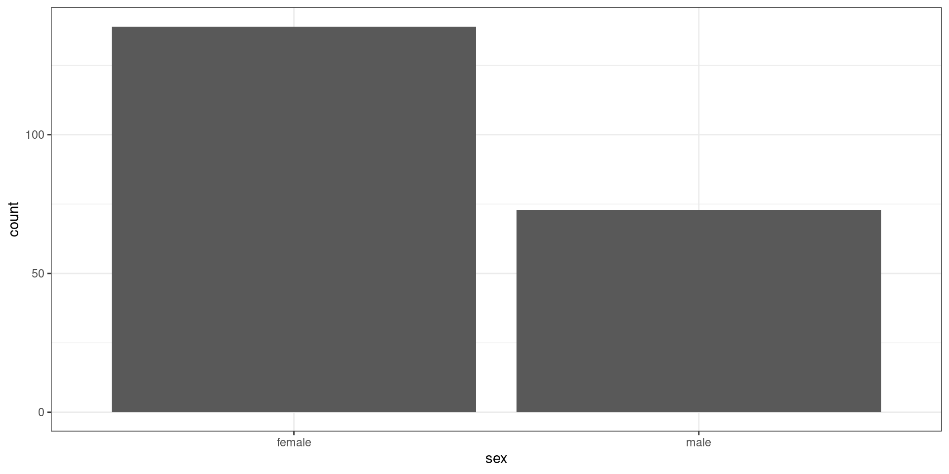
Nominal data
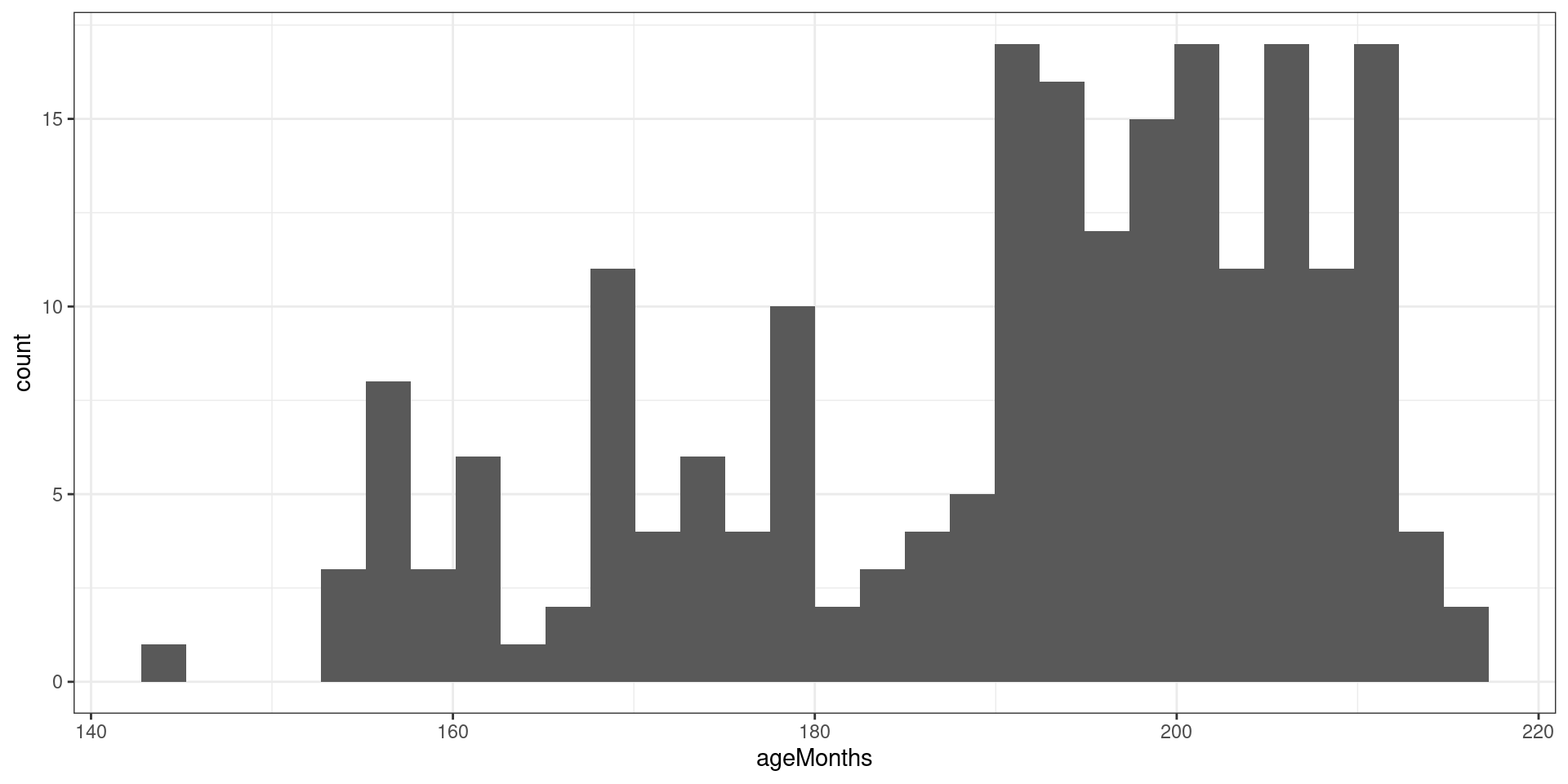
Continuous data
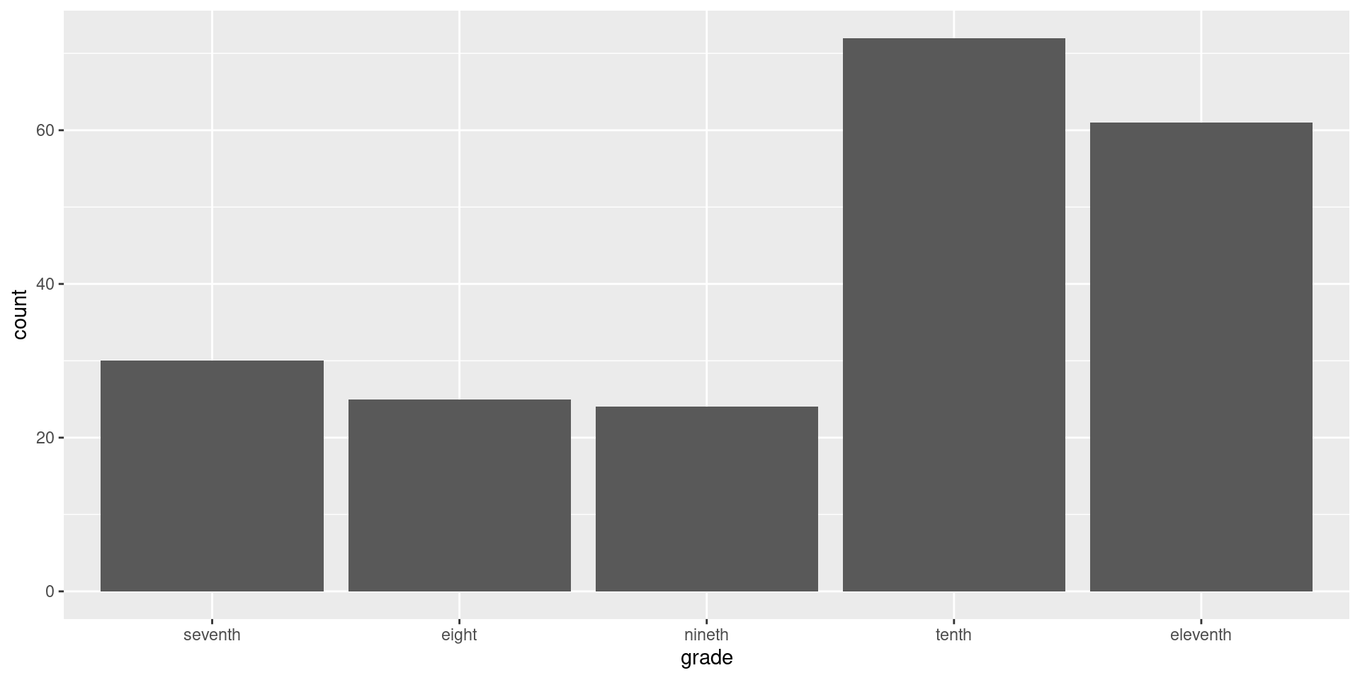
Ordinal data
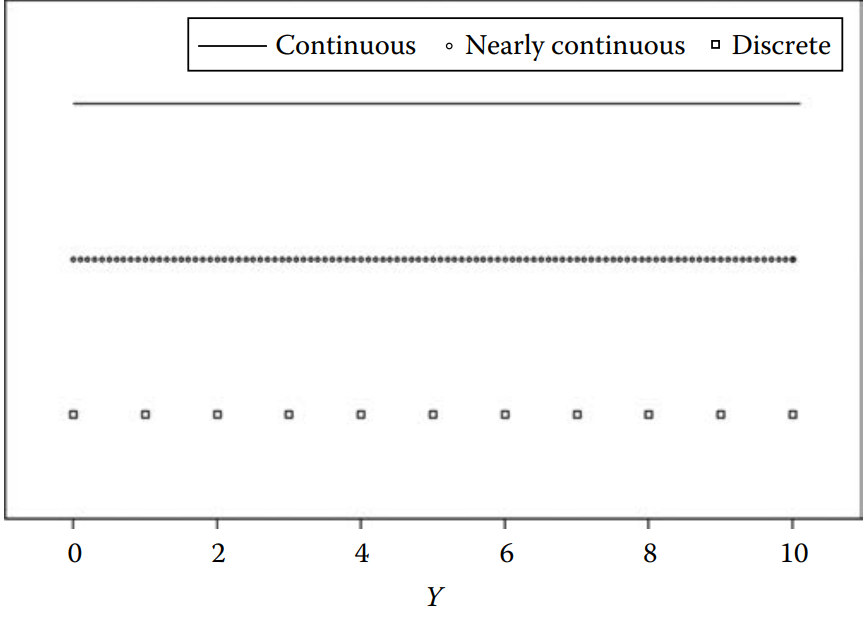
Discrete vs. Continuous
Nominal and Ordinal DATA are considered discrete DATA, this means that values can be listed.
Continuous DATA cannot be listed because all possible values lie in a continuum.
Discrete Probability Distribution Functions
But let’s focus on discrete distributions first.
As I said before, a discrete variable can be listed as showed below:
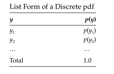
- In this table \(p(y)\) represents the probability of any variable \(y\).
- When we talk about discrete distributions we talk about probability mass function , when the variable is continuous we used the concept probability density function.
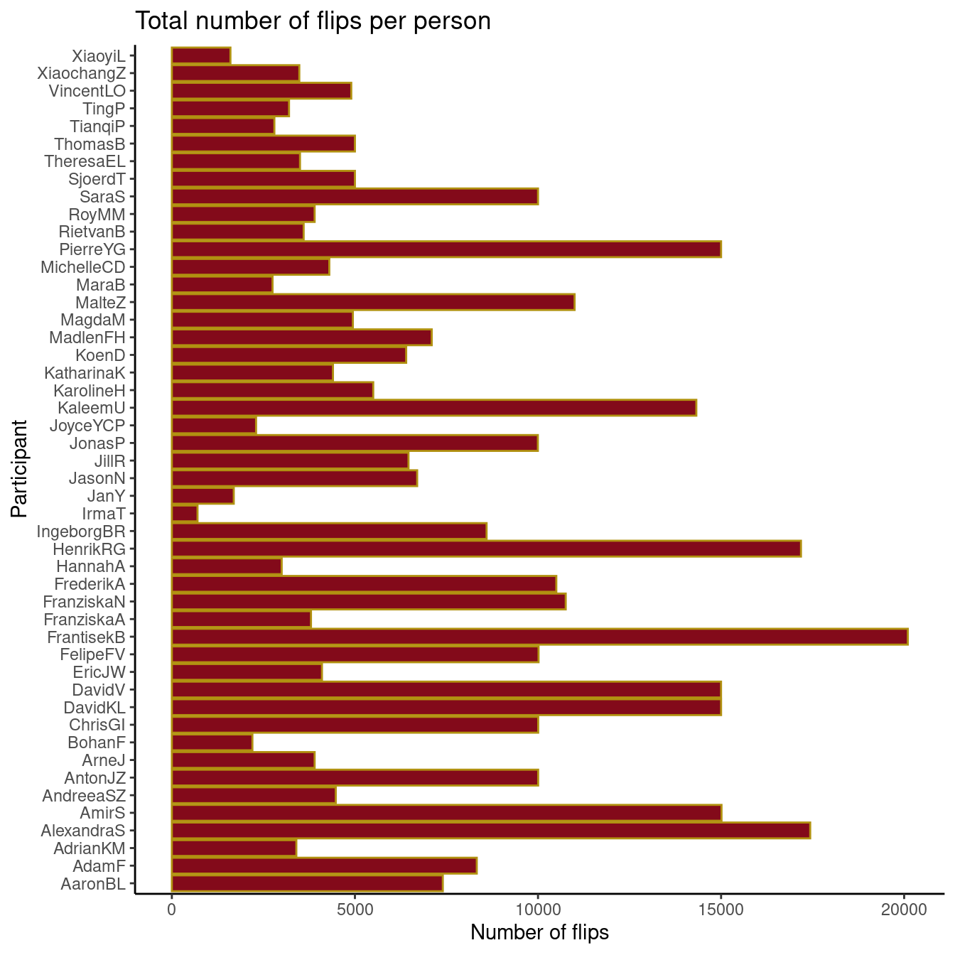
Bartoš et al. (2023) tested several questions associated to flipping coins.
Several participants flipped coins up to a total of 350,757 flips.
Let’s play with their data.
How many times will the coin land on the same side as where it started?

We don’t simulate fliping coins all the time…
We don’t simulate fliping coins all the time…
Show the code
library(tidyverse)

flipsData <- flipsData |>
  mutate(proportionSame = same / flips)

ggplot(flipsData, aes(x=proportionSame)) +
   geom_density(fill = "#00609C", alpha =  0.3)+
  geom_histogram(color = "#B19110",
                 fill= "#830A1A",
                 bins = 10)+
  theme_classic()+
  ggtitle("Histogram of proportions of times coin landed on the same side as where it started")+
  ylab("Frequencies")+
  xlab("Proportions")+
  annotate("text", x = 0.56, y = 30, label = "Mean = 0.51, SD = 0.02")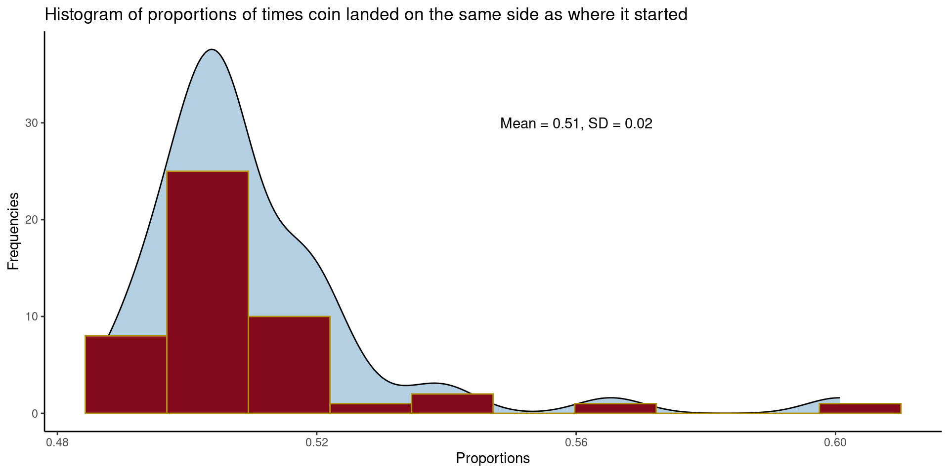
We can return to our simulations …

Simulation time! IV
The probability of each value in our tiny Poisson simulation can be represented in list form as:
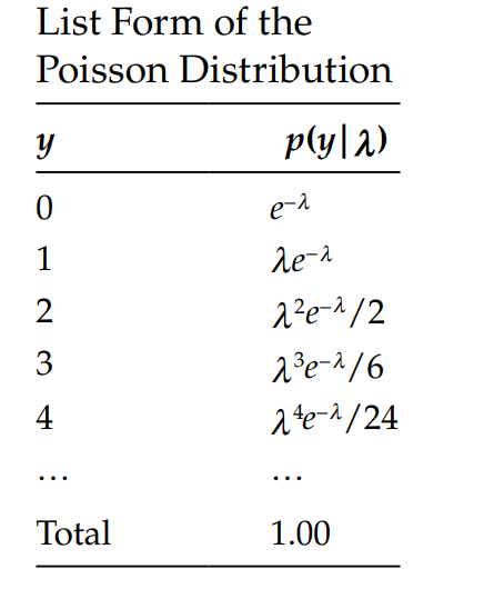
- The Poisson pdf is a good model to represent counts such as the number of times you successfully wake up early and do exercise, the number of shoes, the number of family members in each household and many other counting variables.
Continuous Probability Distribution Functions
- Continuous distributions have several differences compare to discrete distributions.
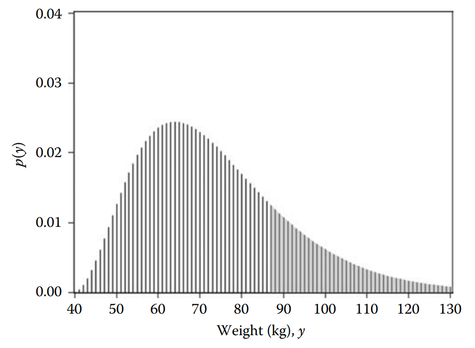
- When the density plot corresponds to a continuous distribution, the \(y\)-axis does not show probability.
- When you estimate the density of continuous distribution you are estimating the “relative likelihood” For example, in this plot 50 kg has a likelihood of around 0.014, 55 kg has a likelihood of around 0.021. This means that is more likely to observe 55 kg compare to 50 kg.
Continuous Probability Distribution Functions II
Important: - The probability of a value in a density plot can only be estimated by calculating by estimating the area under the curve.
- The total area under the curve in discrete and continuous functions is always equal to 1.0.
Continuous Probability Distribution Functions III
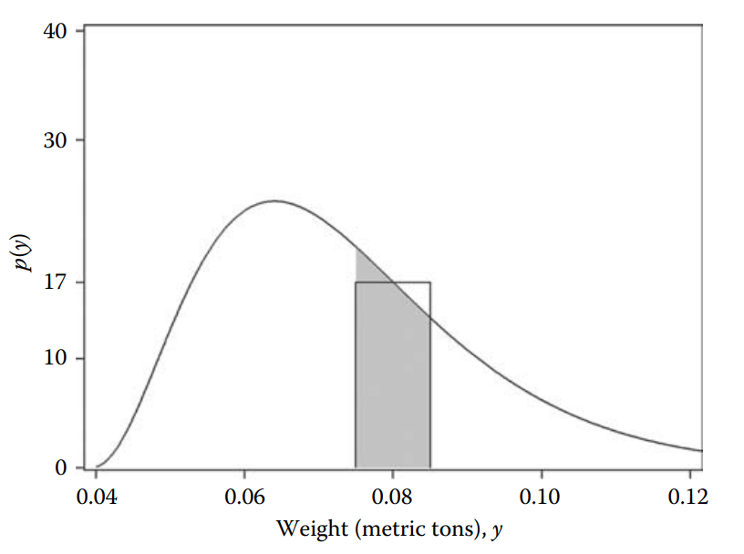
In this graph Westfall & Henning (2013) changed the metric from kg to metric tons.
This helps to show you how to estimate the probability of 0.08 metric tons from a density plot.
Then the probability of observing a weight (in metric tons) in the range \(0.08 \pm 0.005\) is approximately 17 × 0.01 = 0.17. Or in other words, about 17 out of 100 people will weigh between 0.075 and 0.085 metric tons, equivalently, between 75 and 85 kg.
But this is is just an approximation, integrals would give us the exact probability, but we will avoid calculus today.
More distributions: normal distribution III
- We can check the density distribution of this sample that comes from the normal distribution model:

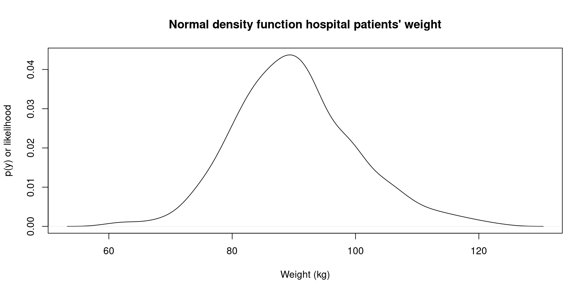
More distributions: normal distribution IV
- We can check now the probability density function of our simulated hospital sample:
More distributions: normal distribution V
library(ggplot2) ### <- this is a package in R to create pretty plots.

dataMerged <- data.frame(
  group =c(rep("College", 300),
           rep("Hospital", 300)),
  weight = c(data_1, data_2))

ggplot(dataMerged , aes(x=weight, fill=group)) +
  geom_density(alpha=.25) +
  theme_bw()+
  labs(title = "College and Hospital Weight Density Function") +
  xlab("Weight (kg)") +
  ylab("p(y) or likelihood")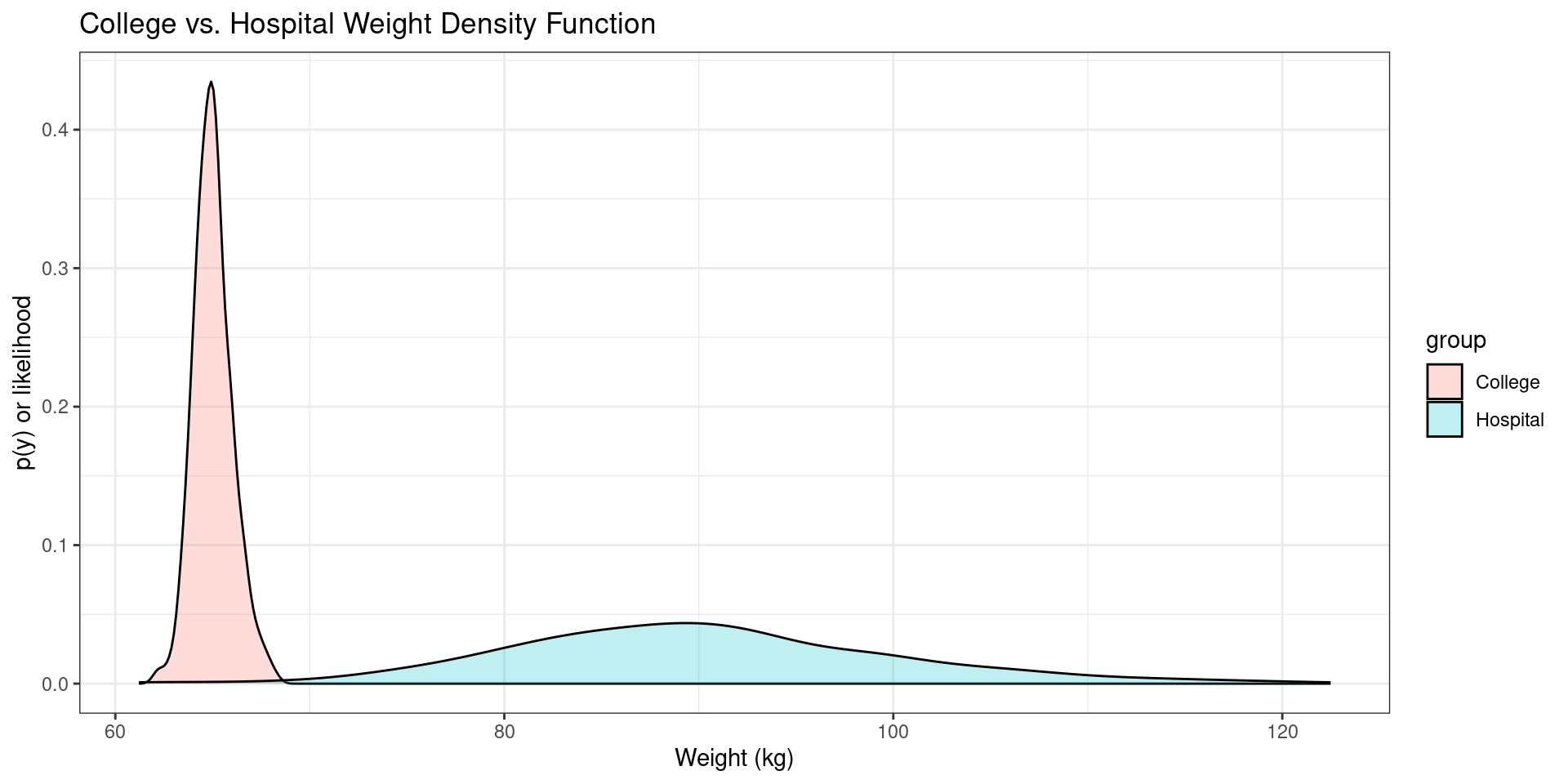
References
![]()
