rum <- read.csv("ruminationComplete.csv", na.string = "99") ## Imports the data into R
rum_scores <- rum %>% mutate(rumination = rowSums(across(CRQS1:CRSQ13)),
depression = rowSums(across(CDI1:CDI26))) ### I'm calculating
## total scores
corr <- cor(rum_scores$rumination, rum_scores$depression,
use = "pairwise.complete.obs") ## Correlation between rumination and depression
### Let's create a distribution of null correlations
nsim <- 100000
cor.c <- vector(mode = "numeric", length = nsim)
for(i in 1:nsim){
depre <- sample(rum_scores$depression,
212,
replace = TRUE)
rumia <- sample(rum_scores$rumination,
212,
replace = TRUE)
cor.c[i] <- cor(depre, rumia, use = "pairwise.complete.obs")
}
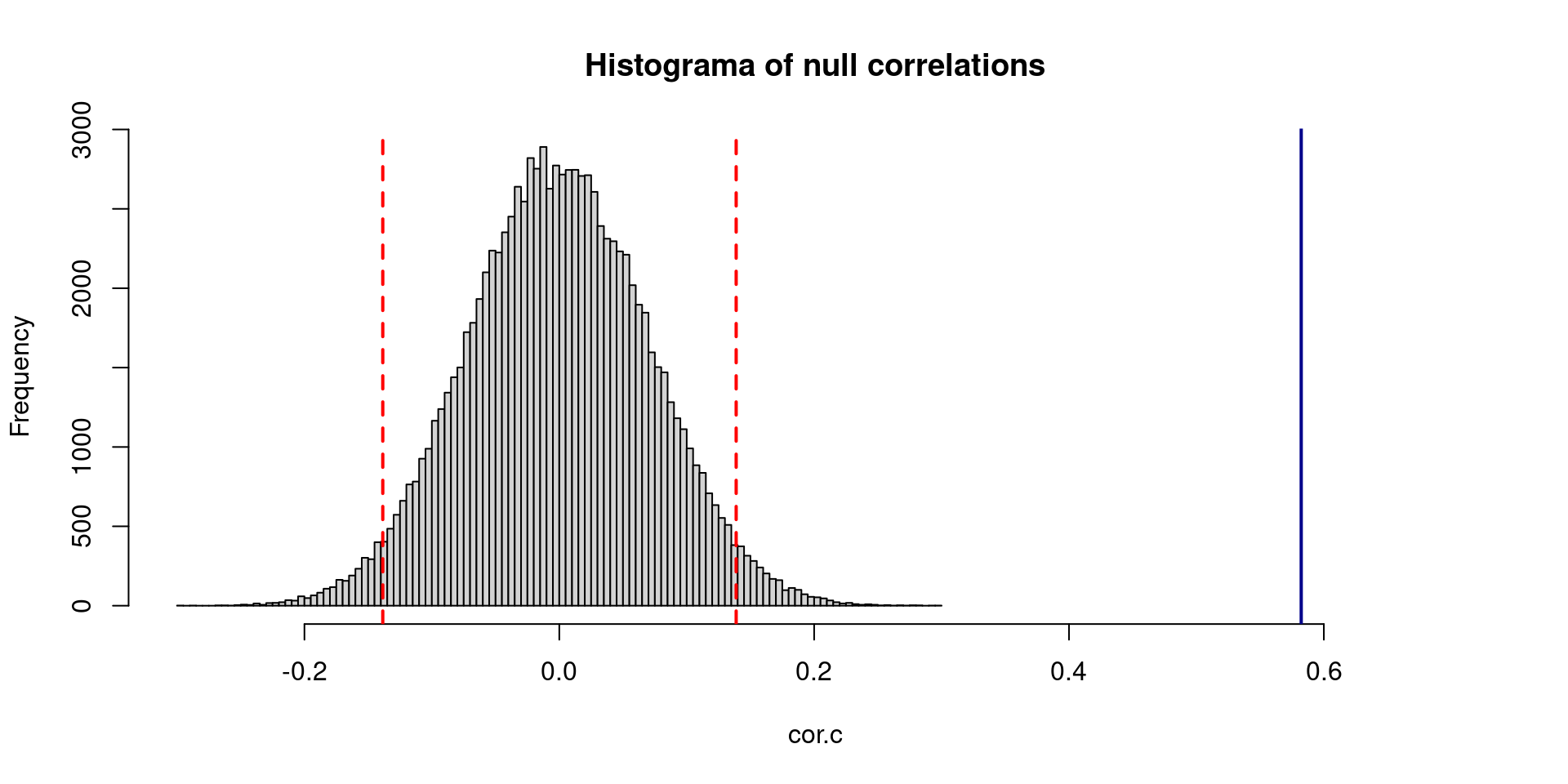
hist(cor.c, breaks = 120,
xlim= c(min(cor.c), 0.70),
main = "Histograma of null correlations")
abline(v = corr, col = "darkblue", lwd = 2, lty = 1)
abline(v = c(quantile(cor.c, .025),quantile(cor.c, .975) ),
col= "red",
lty = 2,
lwd = 2)Compare means and many more stories
What is a p-value? IV
- Let’s see the following example, remember the estimated correlation between rumination and depression is \(r= 0.58\). This null model will help us to know if the correlation is explained by chance.
\(t\)-Test III
- Remember we talked about the \(t\)-distribution’s CDF. This CDF will help us to estimate the probability of seeing a value. the y-axis represents probability values.
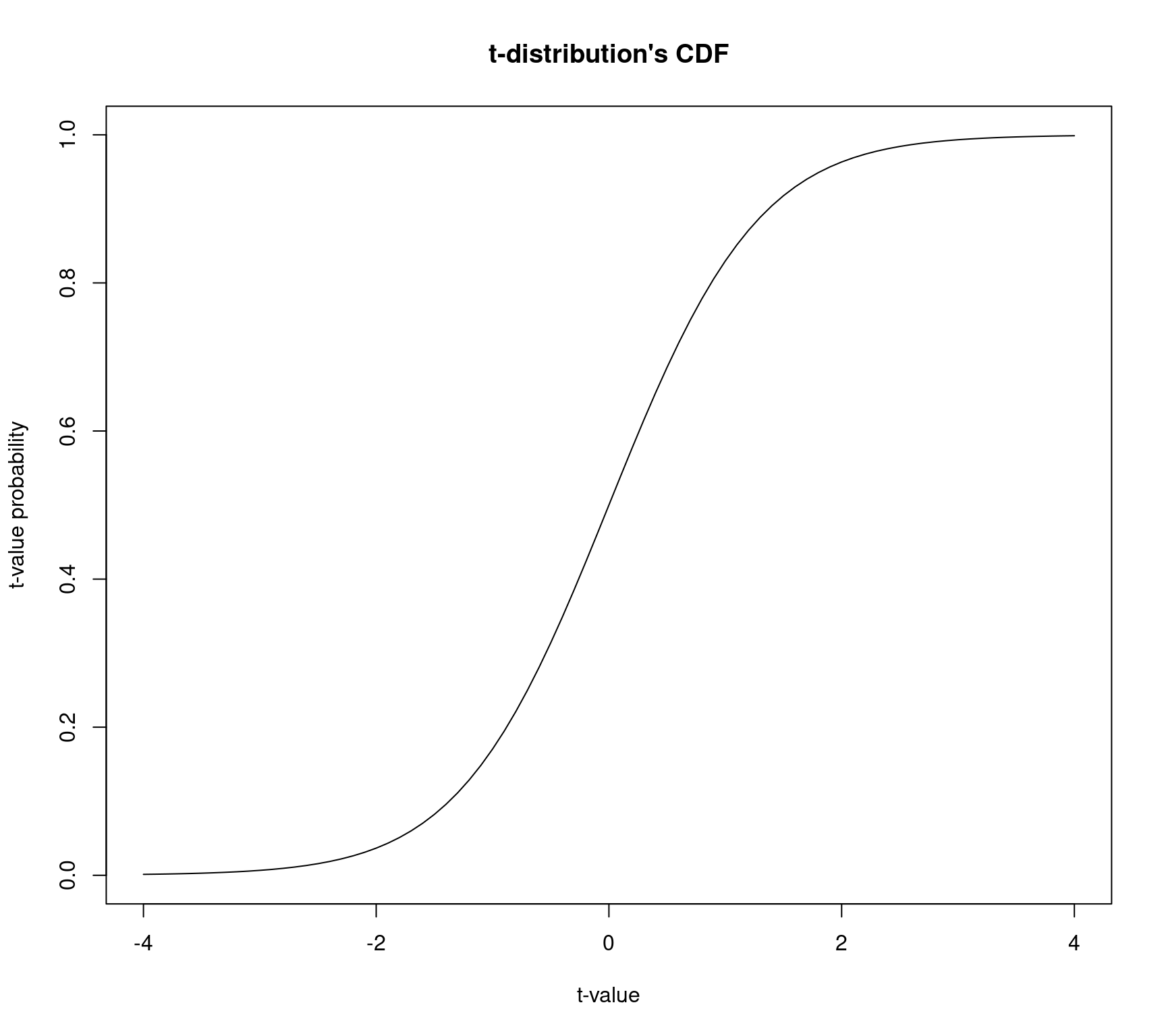
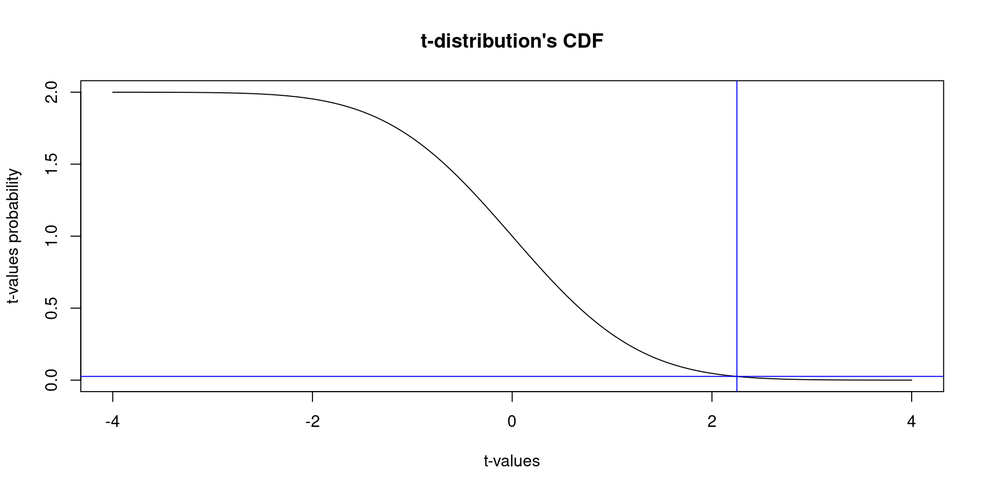
\(t\)-Test IV
We can see how useful is a \(t\)-test by presenting a applied example.
In this example we will try to reject the null hypothesis that says:
The rumination score in males is equal to the rumination score in females
- We represent this hypothesis in statistics like this:
Also in this example I’m introducing a new function in
Rnamedt.test(). This is the function that will helps to know if we can reject the null hypothesis.The function
t.test()requires a formula created by using tilde~.In
Rthe the variable on the right side of~is the independent variable, the variable on the left side of~is the dependent variable.In a independent samples \(t\)-test the independent variable is always the group, and the dependent variable is always any continuous variable.
    Two Sample t-test

data:  rumination by sex
t = 2.2457, df = 203, p-value = 0.0258
alternative hypothesis: true difference in means between group 0 and group 1 is not equal to 0
95 percent confidence interval:
 0.3347849 5.1535481
sample estimates:
mean in group 0 mean in group 1
31.20896 28.46479 - In this example, we found that the \(p\)-value is 0.03 and the \(t\)-value is 2.25. This means:
***“IF we repeat the same analysis with multiple samples the probability of finding a*** \(t\)-value = 2.25 is p = 0.03, under the assumptions of the null model”.
- This is a very small probability, what do you think? Is 2.25 a value explainable by chance alone?
JAMOVI
I hope you remember JAMOVI. I mentioned this software in the first class.
It is also listed in the syllabus.
This is a software that runs
Rusing a interface that does not require to write theRcode. JAMOVI will write theRcode for you behind scenes, it also runs the code for you. Pretty awesome isn’t it?

Central Limit Theorem (CLT) (cont.)
In this example I’ll generate 1000 “datasets” from a Gaussian process (normal distribution) with M = 60, sd = 100. Each data set will contain 10 observations.
After generating 1000 data sets, I’m estimating the mean of those simulated values.
Imagine you are asking the question how many minutes do you need to take a shower? to 10 participants, you then conduct the same study the next day with a different set of 10 participants every day until you get 1000 sets of 10 participants.
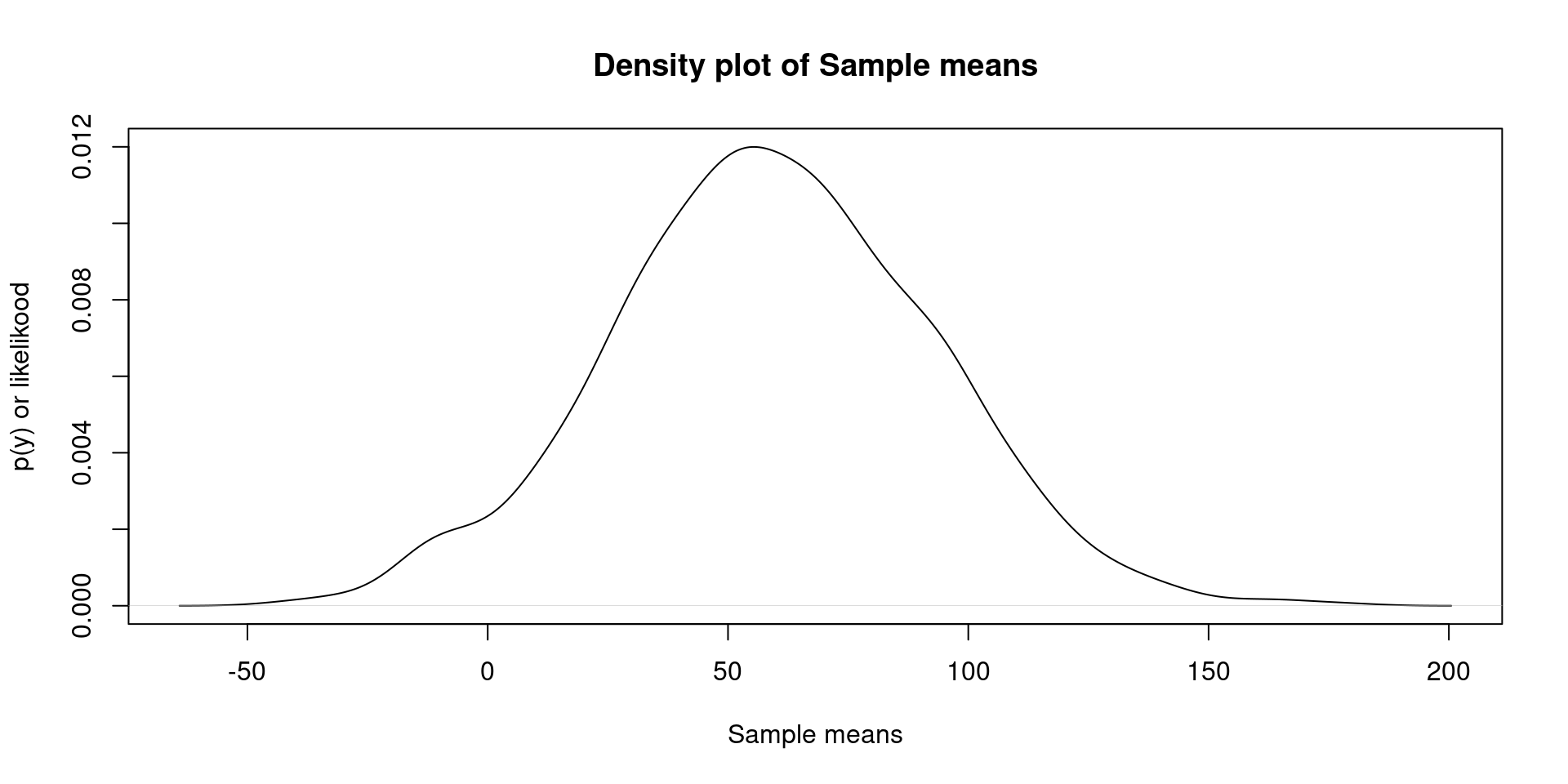
Central Limit Theorem (CLT) (cont.)
There is more beautiful qualities about the CLT. This rule applies to all distributions. When you increase the number of observations per sample, and the number of sample approach infinity. The sample of means will look Gaussian distributed (normally distributed).
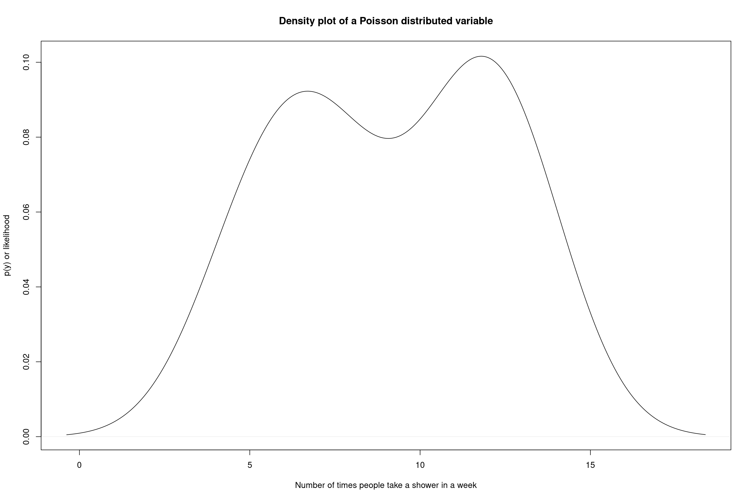
Remember the Poisson distribution I mentioned some lectures behind?
As you can see the Poisson distribution after generating 1 data set of 10 observations doesn’t look like a Gaussian process at all!
Can the sample of means from a Poisson process generate a pretty bell shape?
Central Limit Theorem (CLT) (cont.)
- Let’s find out the answer by simulating 1000 data sets:
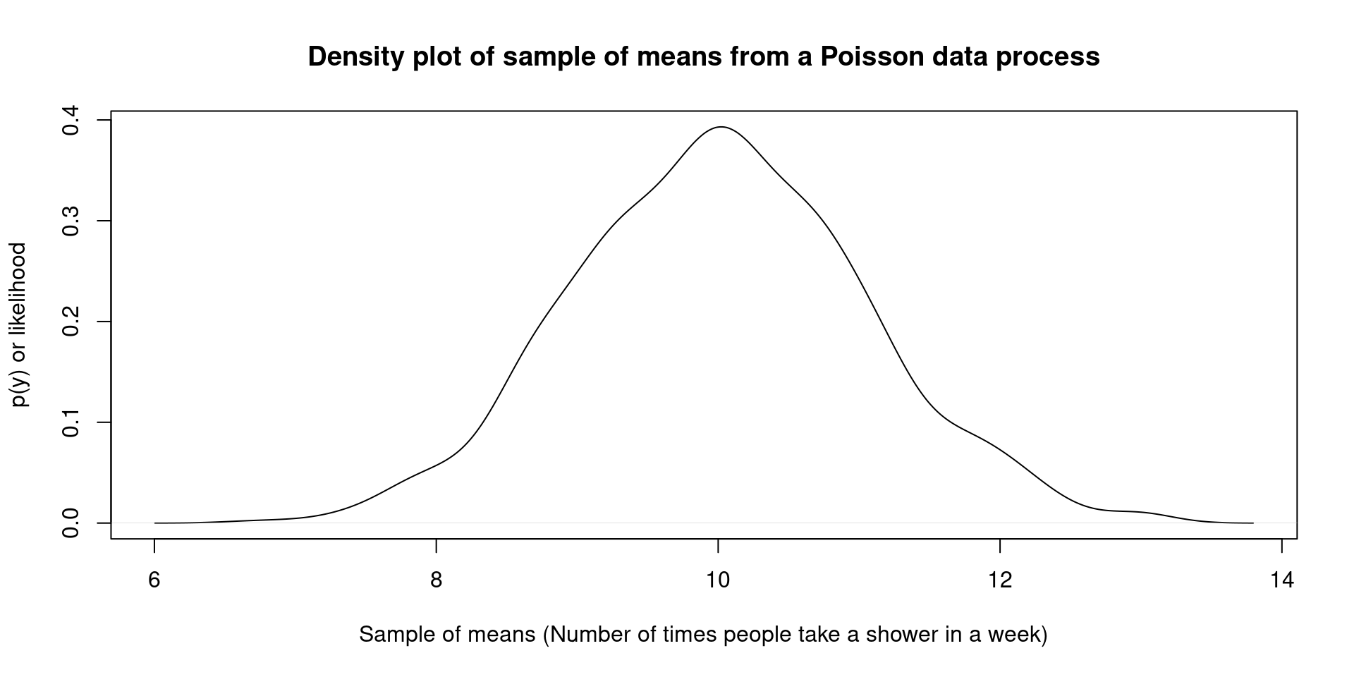
- There is also something even prettier, the mean estimated with all the means, is actually close to the data generating process. It is lovely! This is a natural rule!
Standard Error (cont.)
In real life, you’ll never know the standard deviation of sample means, because this is a simulated example.
In real application you need to estimate how far your observed mean is from the true mean.
We can use this estimation \(\frac{\sigma}{\sqrt(n)}\) to approximate how far we are from the mean. In this formula \(\sigma\) is the standard deviation and \(n\) is the sample size.
The standard error decreases when we increase the sample size, let’s see another example:
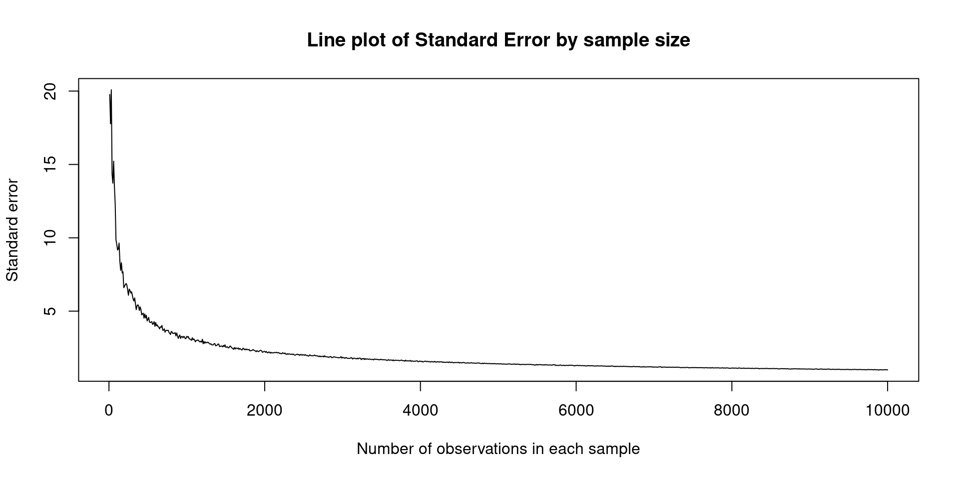
Important
In simple words: The standard error (SE) measures the distance from the true value in the data generating process.
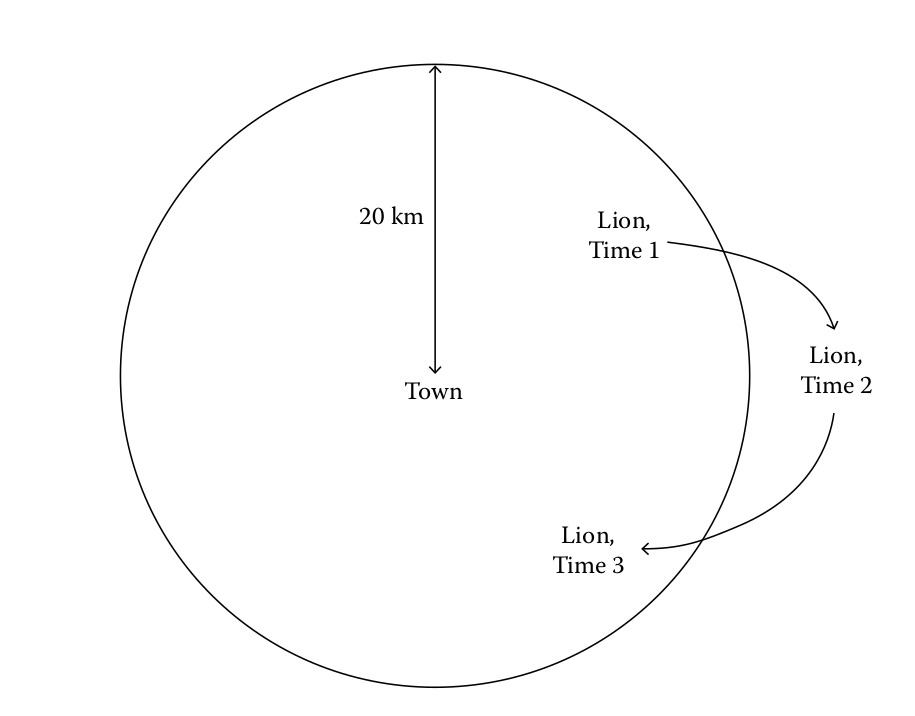
Allow me to use a metaphor
Westfall & Henning (2013):
- Imagine there is a lion or perhaps a coyote around your town. Every day the coyote moves around 20 km from the town, forming a circular perimeter. The town is right in the middle of the circle:
Confidence Interval: multiple means
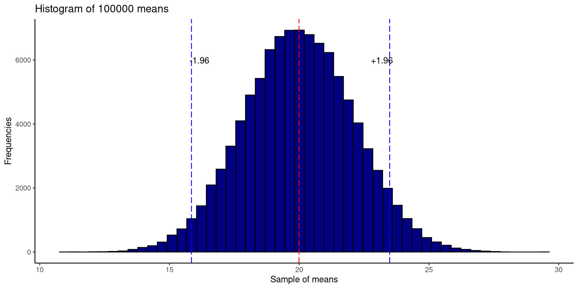
- Let’s imagine a ask the same question: how many minutes do you need to take a shower?
- We could ask the same question to 50 different people 100 000 times, and then estimate the mean. The frequentist theory says that the true value will be among the 95\(\%\) of the sampled means.
References
![]()

Westfall, P. H., & Henning, K. S. (2013). Understanding advanced statistical methods. CRC Press Boca Raton, FL, USA: