#|echo: FALSE
#|eval: TRUE
#|fig-height: 3
#|fig-width: 3
library(ggplot2)
set.seed(1236)
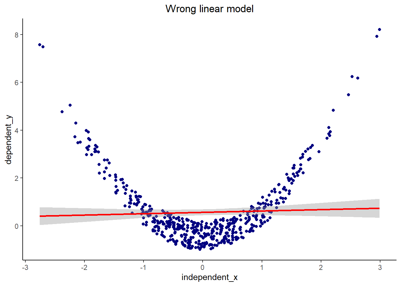
X <- rnorm(500, 0, 1) # simulate from the normal distribution
Y <- X^2 + runif(500, -0.99, 0.20) # make it squared +/- a little bit
dat <- data.frame(independent_x = X,
dependent_y = Y)
ggplot(aes(x=independent_x, y= dependent_y), data=dat ) +
geom_point(color = "navy")+
geom_smooth(method = lm, color = "red")+
ggtitle("Wrong linear model") +
theme_classic()+
theme(plot.title = element_text(hjust = 0.5))`geom_smooth()` using formula = 'y ~ x'