Non-linearity in the classical regression model and basics on moderation
Department of Psychology and Child Development
The world can be non-linear
At this point you probably remember the notion of linearity in the Classical Regression Model.
It is a important assumption in the Classical Regression Model, but it is not a strict assumption. This is a good characteristic of the linear model.
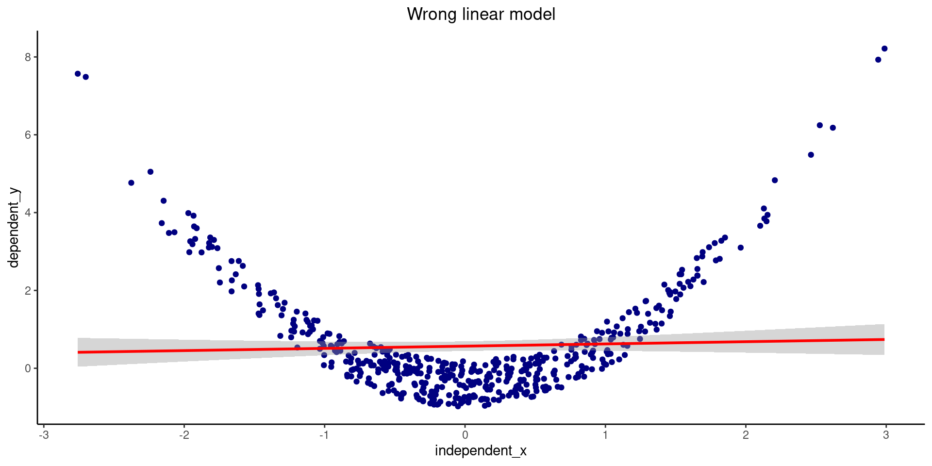
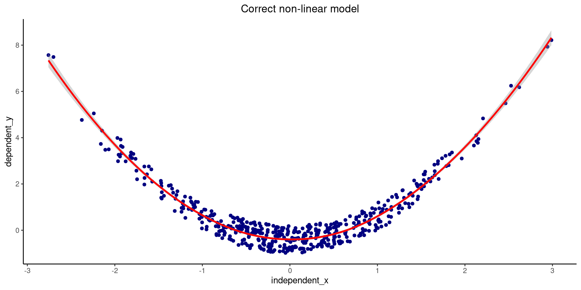
Multiple phenomena in the universe are not linear such as growing curves, or developing curves in human beings are many times not linear at all.
For example, we could check a case where we select the wrong model for the data, like the one showed below:
The world can show you interactions
Regression models are flexible in terms of interactions.
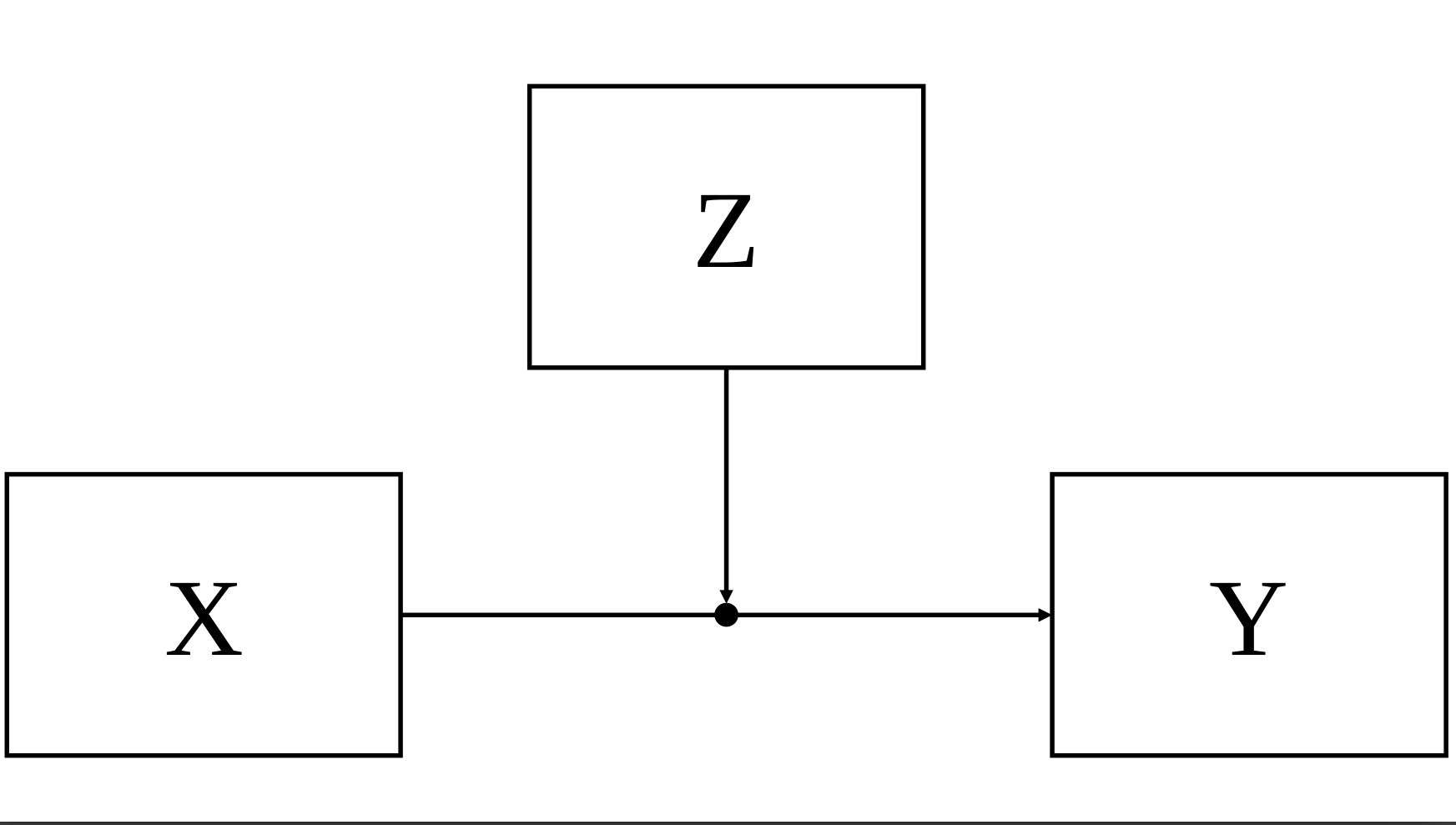
But, what is an interaction?: An interaction is what we call a moderated effect. Let’s see how it looks like:
You can see in (Figure 1) there is a third variable Z affecting the relationship between X and Y. When this happens we say that the relationship between X and Y DEPENDS on Z
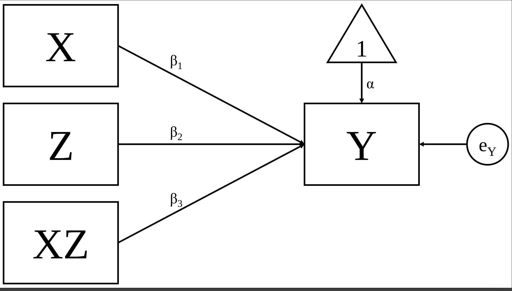
When we analyze an interaction we are estimating the product of a multiplication.
We can represent the Figure 2 in its mathematical form:
\[Y= \alpha + \beta_{1}X + \beta_{2}Z + \beta_{3}XZ + \epsilon_{i}\]
How do we know we should add a moderation term?
- The first step is to test if we need a moderation term in our equation1 .
- We can test it by estimating a regression model.
Show the code
library(haven)
library(parameters)

#### continuous moderation
## stress:
## socsup: social support
## dep: depression
## stressXss: interaction stress * social support
##

url <- "https://raw.githubusercontent.com/blackhill86/mm2/refs/heads/main/dataSets/moderationExample.csv"


stress <- read.csv(url)

### Regression model without interaction
fitModel_1 <- lm(dep ~ socsup + stress,
                 data=stress)

model_parameters(fitModel_1,
                 verbose = FALSE)
Parameter | Coefficient | SE | 95% CI | t(138) | p
-------------------------------------------------------------------
(Intercept) | 12.75 | 2.52 | [ 7.77, 17.74] | 5.06 | < .001
socsup | -0.43 | 0.12 | [-0.66, -0.20] | -3.71 | < .001
stress | 0.13 | 0.03 | [ 0.08, 0.19] | 4.87 | < .001In the model above, I’m testing if social support and stress are related to depression.
The model looks like this:
\[Y= \alpha + \beta_{1}Stress + \beta_{2}SocialSupport + e_{i}\]
- Given that the p-value is smaller than 0.05 (\(\le .05\)) we can conclude that the relationship of depression with social support and stress is not explained by chance alone. But, do we need to add an interaction term? Let’s test if a interaction term is explainable by chance:
\[Y= \alpha + \beta_{1}Stress + \beta_{2}SocialSupport + \beta_{3}Stress*SocialSupport + e_{i}\]
Show the code
Parameter       | Coefficient |       SE |         95% CI | t(137) |      p
---------------------------------------------------------------------------
(Intercept)     |        1.81 |     4.77 | [-7.63, 11.25] |   0.38 | 0.705
socsup          |        0.11 |     0.23 | [-0.35,  0.57] |   0.48 | 0.635
stress          |        0.48 |     0.13 | [ 0.22,  0.75] |   3.63 | < .001
socsup × stress |       -0.02 | 6.47e-03 | [-0.03,  0.00] |  -2.68 | 0.008
The interaction term is not explained by chance because \(p= 0.008\) which is less than \(0.05\).
If you find that a interaction terms is not explained by chance, you CANNOT interpret the individual terms because they are MODIFIED or DEPEND on Z.
How do you interpret an interaction effect ?
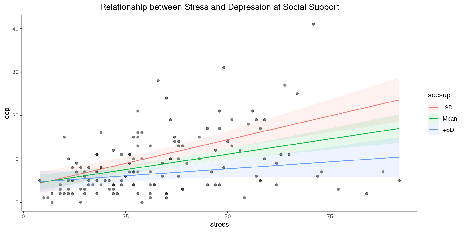
The interpretation can be a little bit tricky. First, we need to understand the relation between depression and stress at each level of our moderator.
In our example, I selected social support as our moderator:
How do you interpret an interaction effect ?
Show the code
library(marginaleffects)
library(ggplot2)

### WE can use the package marginaleffects to
### generate slopes at different levels of
### the moderator

plot_predictions(fitModel_2,
                 condition = list("stress",
                                  "socsup" = "threenum" ),
                 points = 0.5) +
  theme_classic()+
  ggtitle("Relationship between Stress and Depression at Social Support")+
  theme(plot.title = element_text(hjust = 0.5))
Let’s talk about simple slopes
It is also named pick-a-point or spotlight analysis.
In this approach we can select any value from our moderator, and test the conditional effect of \(X\) on \(Y\).
I apologize but you will see some math here:
- You may remember our moderated equation:
\[Y= \alpha + \beta_{1}X + \beta_{2}Z + \beta_{3}XZ + \epsilon_{i}\] - We can reorder terms to get back to this:
\[Y= \alpha + (\beta_{1} + \beta_{3}Z)X + \beta_{2}Z + \epsilon\]
- This re-organization will help us to formulate the next function:
\[f(Z)=\beta_{1} + \beta_{3}Z\] \(f(Z)\) is actually our simple slope. By plugging different values of \(Z\) into \(f(Z)\), we get the slope of the conditional effect of \(X\) on \(Y\) at the chosen value of \(Z\).
Simple slopes estimation
The most popular choices to plug in here: \(f(Z)=\beta_{1} + \beta_{3}Z\), are \(+1SD\), the mean, and \(-1SD\) corresponding to our moderator \(Z\).
We don’t have to estimate these simple slopes “by-hand”, we can estimate different regression models after centering at the critical values we want to test.
Simple slopes estimation: centering
Centering transforms a variable by subtracting a constant (e.g., the variable’s mean) from each observation of the variable.
The most familiar form of center is mean centering We can center on any value.
When probing interactions, we can center \(Z\) on the interesting values we choose during the pick-a-point approach.
Running the model with \(Z\) centered on specific values automatically provides tests of the simple slope conditional on those values of \(Z\).
Simple slopes estimation: centering
- In our example, the moderator is social support. We can center our moderator at the mean, 1 SD above the mean, and 1 SD below the mean.
-In the following R chunk, I’ll create three new variables in the object stress which contains my data information. The three new variables are:
- SocialMean = \(socialSupport_{i} - mean(SocialSupport)\)
- SocialHigh = \(socialSupport_{i} - (mean(SocialSupport)+ sd(SocialSupport))\)
- SocialLow = \(socialSupport_{i} - (mean(SocialSupport) - sd(SocialSupport))\)
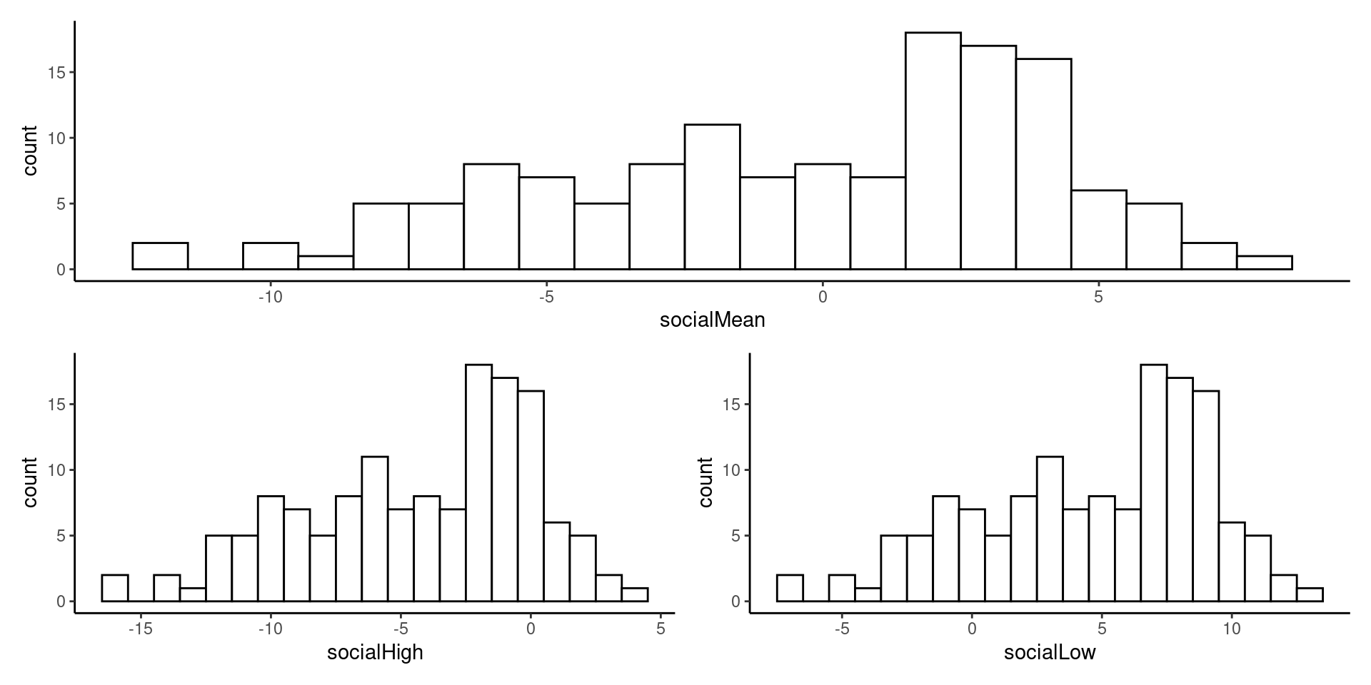
- Let’s check the new variables with a histogram:
Show the code
library(patchwork)

atMean <- ggplot(aes(x=socialMean), data = stress) +
  geom_histogram(colour = 1,
                 fill = "white",
                 binwidth = 1) +
  theme_classic()

atHigh <- ggplot(aes(x=socialHigh), data = stress) +
  geom_histogram(colour = 1,
                 fill = "white",
                 binwidth = 1) +
  theme_classic()

atLow <- ggplot(aes(x=socialLow), data = stress) +
  geom_histogram(colour = 1,
                 fill = "white",
                 binwidth = 1) +
  theme_classic()

atMean/(atHigh+atLow)- Now, we can use this three new computed centered variables to estimate our simple slopes at the mean, \(mean + 1SD\), and \(mean - 1SD\).
Simple slopes estimation time
With our new computed variables we can now test our simple slopes, we will estimate a regression model for each simple slope. This will help us to test if the simple slope is explainable by chance.
First simple slope at the mean:
Show the code
Parameter           | Coefficient |       SE |         95% CI | t(137) |      p
-------------------------------------------------------------------------------
(Intercept)         |        3.99 |     1.02 | [ 1.97,  6.01] |   3.91 | < .001
stress              |        0.14 |     0.03 | [ 0.09,  0.19] |   5.24 | < .001
socialMean          |        0.11 |     0.23 | [-0.35,  0.57] |   0.48 | 0.635
stress × socialMean |       -0.02 | 6.47e-03 | [-0.03,  0.00] |  -2.68 | 0.008
When estimating a model with a centered moderator, the slope of your predictor, in this case stress becomes your estimated simple slope. In our example the simple slope at the mean of social support is: \(\beta=0.14\), and it is not explained by chance because the p-value is less than 0.05.
Second simple slope at high values of social support:
Show the code
Parameter           | Coefficient |       SE |         95% CI | t(137) |     p
------------------------------------------------------------------------------
(Intercept)         |        4.48 |     1.39 | [ 1.74,  7.22] |   3.23 | 0.002
stress              |        0.06 |     0.04 | [-0.01,  0.14] |   1.73 | 0.086
socialHigh          |        0.11 |     0.23 | [-0.35,  0.57] |   0.48 | 0.635
stress × socialHigh |       -0.02 | 6.47e-03 | [-0.03,  0.00] |  -2.68 | 0.008
In the case of the simple slope at the high level of social support is \(\beta = 0.06\), and it is explained by chance because the p-value is greater than \(0.05\).
Third simple slope at low values of social support:
Show the code
Parameter          | Coefficient |       SE |         95% CI | t(137) |      p
------------------------------------------------------------------------------
(Intercept)        |        3.50 |     1.51 | [ 0.50,  6.49] |   2.31 | 0.022
stress             |        0.22 |     0.04 | [ 0.14,  0.30] |   5.26 | < .001
socialLow          |        0.11 |     0.23 | [-0.35,  0.57] |   0.48 | 0.635
stress × socialLow | -0.02 | 6.47e-03 | [-0.03, 0.00] | -2.68 | 0.008 - In the third simple slope, the estimated value is \(\beta = 0.22\), and it is not easy to explain this slope by chance because the p-value is much less than 0.05.
Simple slopes interpretation time
In our model depression is our outcome, stress our predictor, and social support our moderator. After estimating our simple slopes at different levels of our moderator we can conclude the following:
The effect of stress on depression is stronger when participants have a low level of social support: \(\beta = 0.22\).
The effect of stress on depression gets weaker when participants are close to the mean of social support: \(\beta= 0.14\).
The effect of stress on depression gets much weaker when participants have a high score in social support \(\beta= 0.11\). This simple slope is explained by chance. This means that the relationship between depression and stress is explained by chance when participants have a high social support.
Simple slopes: Johnson-Neyman technique
You may be thinking: what happens if I want to test all the possible values of my moderator?
The answer is the Johnson-Neyman technique.
The Johnson-Neyman technique is an alternative approach that removes the arbitrary choices necessary for pick-a-point.
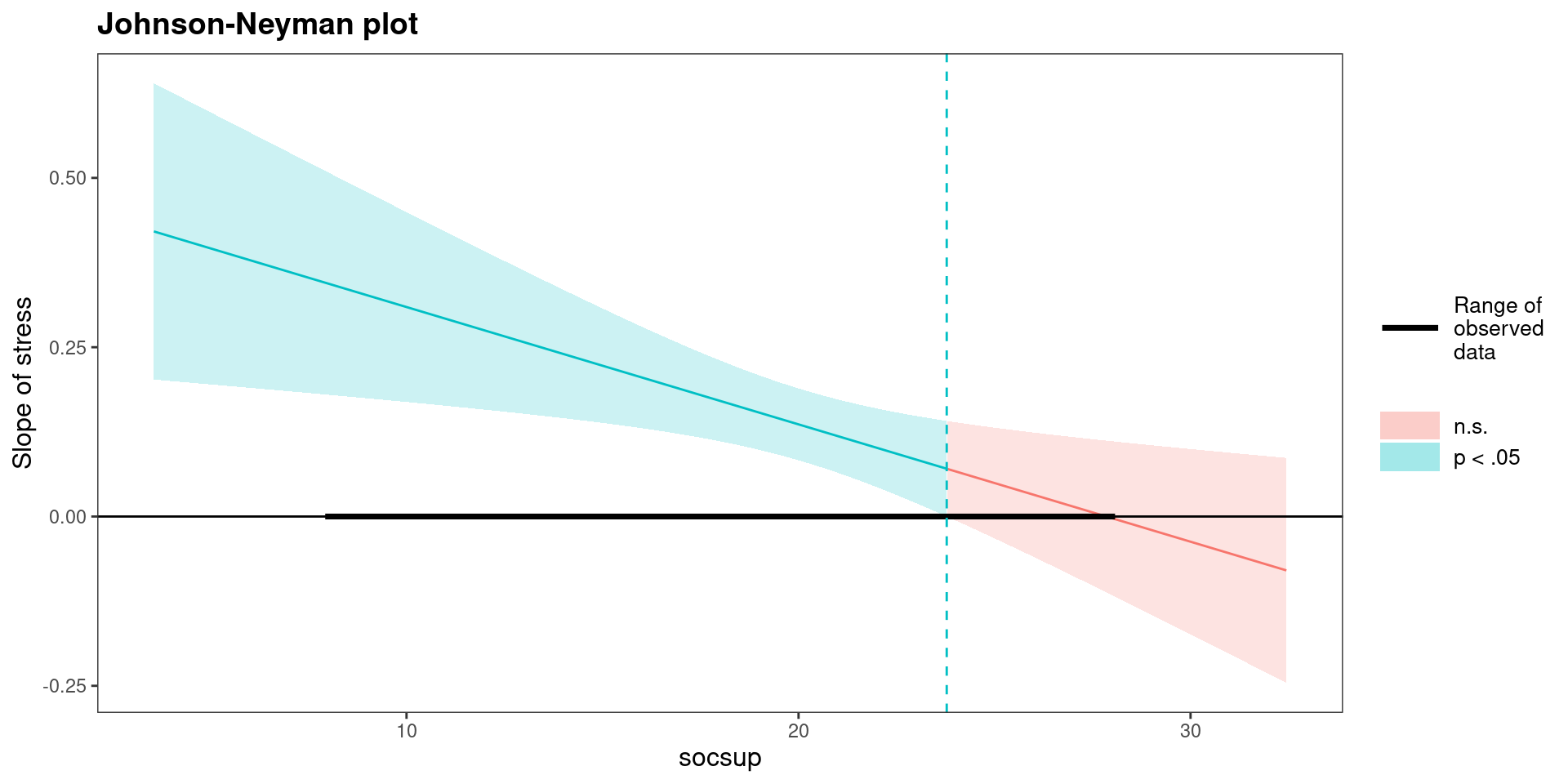
Johnson-Neyman finds the region of significance wherein the conditional effect of \(X\) on \(Y\) is statistically significant.
Inverts the pick-a-point approach to find what cut-points on the moderator correspond to a critical \(t\) value for the conditional \(\beta_{1}\).
This requires to solve a set of equations that I’m not explaining in this lecture but, the simple message is that Johnson-Neyman’s strategy can give you a region of significance accross values of your moderator.
Simple slopes: Johnson-Neyman technique in R
The Johnson-Neyman technique is implemented in the
Rpackagerockchalk. There are more packages performing this strategy.You first need to estimate your moderated regression model, this means a model with at least one interaction term.
Secondly you can estimate the simple slopes, and the region of significance.
Show the code
JOHNSON-NEYMAN INTERVAL

When socsup is OUTSIDE the interval [23.78, 50.44], the slope of stress is
p < .05.

Note: The range of observed values of socsup is [8.00, 28.00]
SIMPLE SLOPES ANALYSIS
Slope of stress when socsup = 15.24283 (- 1 SD):
Est. S.E. t val. p
------ ------ -------- ------
0.22 0.04 5.26 0.00
Slope of stress when socsup = 19.68794 (Mean):
Est. S.E. t val. p
------ ------ -------- ------
0.14 0.03 5.24 0.00
Slope of stress when socsup = 24.13306 (+ 1 SD):
Est. S.E. t val. p
------ ------ -------- ------
0.06 0.04 1.73 0.09Acknowledgement
This lecture was created based on the materials created by Kyle M. Lang (2016) and Mauricio Garnier-Villareal (2020)

