Introduction to Hypothesis Testing

Esteban Montenegro-Montenegro, PhD

Psychology and Child Development

Today’s aims

  • We will study the concept of p-value a.k.a significance test.

  • I will introduce the concept of hypothesis testing.

  • I will also introduce the mean comparison for independent groups.

library(knitr)
library(kableExtra)
library(dplyr)

Attaching package: 'dplyr'
The following object is masked from 'package:kableExtra':

    group_rows
The following objects are masked from 'package:stats':

    filter, lag
The following objects are masked from 'package:base':

    intersect, setdiff, setequal, union
What is a p-value?

  • p-value stands for probability value.

  • It was born as a measure to reject a hypothesis.

  • In statistics and science, we always have hypothesis in mind. Statistics translates our hypothesis into evaluations of our hypothesis.

  • For example, we often ask questions to our selves such as: why my boyfriend won’t express her feelings? and then we ask, is this related to gender? Is it true that women share easily their emotions compare to men? If so, does it happen only to me? Is this a coincidence?

  • We can create a hypothesis with these questions, let’s try to write one:

\(H_{1}\) = There is a difference in emotional expression between cisgender women and cisgender men.

  • This is our alternaive hypothesis but we need a null hypothesis:

\(H_{0}\) = There is no difference in emotional expression between cisgender women and cisgender men.

  • That was easy you might think, but why do we need a null statement?

    • Science always starts with a null believe, and what we do as scientist is to collect evidence that might help to reject the null hypothesis. If you collect data to support your alternative hypothesis you would be doing something called “confirmation bias”.
    • Confirmation bias consist of collecting information that only supports your alternative hypothesis.
    • For example, you start collecting data that only proofs that all swans are white, instead of looking at information that helps to reject the null: not all swans are white.

What is a p-value? II

  • We can write out null hypothesis in a statistical statement:

\(H_{0}\) = The mean difference in emotional expression between cisgender women and cisgender men is equal to zero.

  • In the previous hypothesis we know that we are focusing in the mean difference, it is more specific.

  • The very first step to test our null hypothesis is to create a null model.

  • A null model is a model where there is not any difference between groups, or there is not relationship between variables.

What is a p-value? III

  • In my new model I will find a null model for the correlation between rumination and depression.

  • To create our new model we will re sample and shuffle our observed data. This is similar to have two decks of cards and you shuffle your cards multiple times until it is hard to guess which card will come next, and imagine cards have equal probability to be selected.

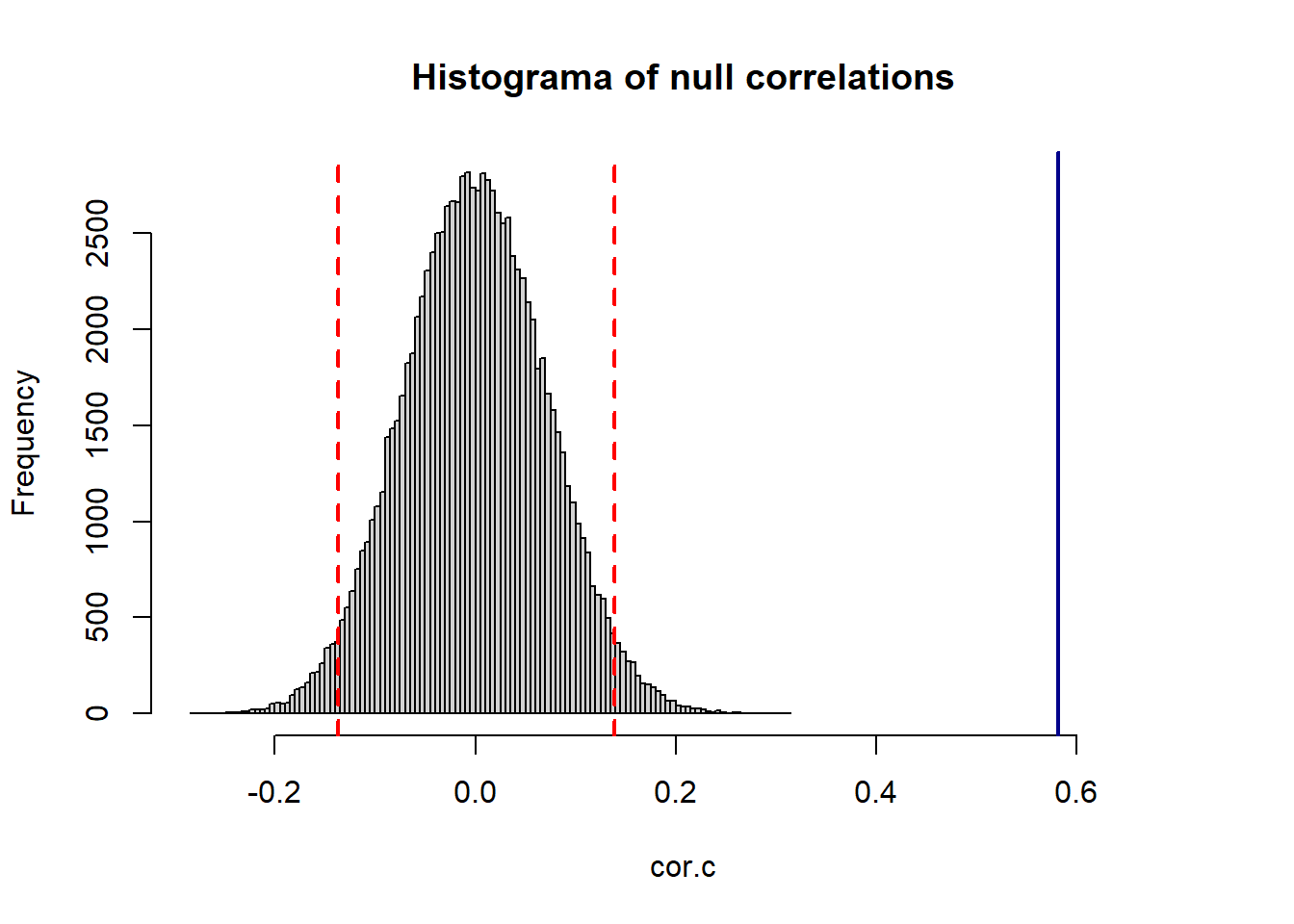
  • This procedure is called permutations, this will help us to create a distribution of null correlations. This means, all the correlations produced by my null model are produced by chance.

What is a p-value? IV

  • Let’s see the following example, remember the estimated correlation between rumination and depression is \(r= 0.58\). This null model will help us to know if the correlation is explained by chance.
rum <- read.csv("ruminationComplete.csv", na.string = "99") ## Imports the data into R

rum_scores <- rum %>% mutate(rumination = rowSums(across(CRQS1:CRSQ13)),
                             depression =  rowSums(across(CDI1:CDI26))) ### I'm calculating
                                                                       ## total scores


corr <- cor(rum_scores$rumination, rum_scores$depression,
            use =  "pairwise.complete.obs") ## Correlation between rumination and depression

### Let's create a distribution of null correlations

nsim <- 100000

cor.c <- vector(mode = "numeric", length = nsim)

for(i in 1:nsim){
depre <- sample(rum_scores$depression, 
                212, 
                replace = TRUE)

rumia <- sample(rum_scores$rumination, 
                212, 
                replace = TRUE)

cor.c[i] <- cor(depre, rumia, use =  "pairwise.complete.obs")
}


hist(cor.c, breaks = 120, 
     xlim= c(min(cor.c), 0.70),
     main = "Histograma of null correlations")
abline(v = corr, col = "darkblue", lwd = 2, lty = 1)
abline(v = c(quantile(cor.c, .025),quantile(cor.c, .975) ),
 col= "red",
 lty = 2,
 lwd = 2)

What is a p-value? V

Let’s estimate the probability of seeing \(r = 0.58\) according to our null model.

pVal <- 2*mean(cor.c >= corr)
pVal
[1] 0
  • The probability is a number close to \(0.00\).

  • We now conclude that a correlation as extreme as \(r = 0.58\) is not explained by chance alone.

Note:

The ugly rule of thumb is to consider a p-value <= .05 as evidence of small probability.

Mean difference

  • We can also do the same for the difference between means.

  • In this example, my null model is a model with null differences.

  • I also conducted permutations on this example.

  • We will estimate if the difference by sex in rumination is explained by chance.

  • In this sample the mean difference in rumination between males and females is \(\Delta M\) = 2.74.

set.seed(1236)

ob.diff <- mean(rum_scores$rumination[rum_scores$sex==0], na.rm = TRUE )- mean(rum_scores$rumination[rum_scores$sex==1], na.rm = TRUE)

### let's create a distribution of null differences

nsim <- 100000

diff.c <- vector(mode = "numeric", length = nsim)

### This is something called "loop", you don't have to pay attention to this.

for(i in 1:nsim){
women <- sample(rum_scores$rumination[rum_scores$sex==0], 
                length(rum_scores$rumination[rum_scores$sex==0]), 
                replace = TRUE)

men <- sample(rum_scores$rumination[rum_scores$sex==1], 
                length(rum_scores$rumination[rum_scores$sex == 1]), 
                replace = TRUE)

diff.c[i] <- mean(women,  na.rm = TRUE)-mean(men,  na.rm = TRUE)
} 


hist(diff.c, breaks = 120, 
     #xlim= c(min(diff.c), 0.70),
     main = "Histogram of Null Differences")
abline(v = ob.diff, col = "darkblue", lwd = 2, lty = 1)
abline(v = c(quantile(diff.c, .025), quantile(diff.c, .975) ),
 col= "red",
 lty = 2,
 lwd = 2)

  • We can see the probability of seeing a value as large as 2.74
pVal <- 2*mean(diff.c >= ob.diff)
pVal
[1] 0.99652

Mean difference II

  • In real life, we don’t have to estimate a null model “by hand” as I did before.

  • R and JAMOVI will help us on that because the null model is already programmed.

  • In addition, when we compare independent means, we don’t usually do permutations. We follow something called the \(t\) - distribution , let’s study more about this distribution: t-distribution.

Mean difference III

  • The \(t\)-distribution helped to develop the test named t-Student Test.

  • In this test we use the \(t\)-distribution as our model to calculate the probability to observe a value as extreme as 2.74.

  • But this probbaility will be estimated following the Cumulative Density Function (CDF) of the \(t\)-distribution.

\(t\)-Test

  • The Student’s test is also known as a the “t-test”.

  • In this test, we will transform the mean difference of both groups into a \(t\) value.

\[\begin{equation} t= \frac{\bar{X}_{1} - \bar{X}_{2}}{\sqrt{\Big [\frac{(n_{1}-1)s^{2}_{1}+(n_{2}-1)s^{2}_{2}}{n_{1} + n_{2}-2}\Big ]\Big [\frac{n_{1}+n_{2}}{n_{1}n_{2}} \Big ]}} \end{equation}\]
  • In this transformation \(n_{1}\) is the sample size for group 1, \(n_{2}\) is the sample size for group 2, \(s^2\) means variance. The \(\bar{X}\) represents the mean.

  • This formula will help us to tranform the oberved difference in means to a value that comes from the \(t\)-distribution.

\(t\)-Test III

  • Remember we talked about the \(t\)-distribution’s CDF. This CDF will help us to estimate the probability of seeing a value. the y-axis represents probability values.
valores <- seq(-4,4, by = 0.1)

probabilidad <- pt(valores, df = 10)

plot(valores, 
     probabilidad, 
     type = "l",
     xlab = "t-value",
     ylab = "t-value probability",
     main = "t-distribution's CDF")

\(t\)-Test IV

  • We can see how useful is a \(t\)-test by presenting a applied example.

  • In this example we will try to reject the null hypothesis that says:

“The rumination score in males is equal to the rumination score in females”

  • We represent this hypothesis in statitistic like this:
\[\begin{equation} H_{0}: \mu_{1} = \mu_{0} \end{equation}\]
  • Also in this example I’m introducing a new function in R named t.test(). This is the function that will helps to know if we can reject the null hypothesis.

  • The function t.test() requires a formula created by using tilde ~.

  • In R the the variable on the right side of ~ is the independent variable, the variable on the left side of ~ is the dependent variable.

  • In a independent samples \(t\)-test the independent variable is always the group, and the dependent variable is always any continuous variable.

t.test(rumination ~ sex, data = rum_scores, var.equal = TRUE)

    Two Sample t-test

data:  rumination by sex
t = 2.2457, df = 203, p-value = 0.0258
alternative hypothesis: true difference in means between group 0 and group 1 is not equal to 0
95 percent confidence interval:
 0.3347849 5.1535481
sample estimates:
mean in group 0 mean in group 1 
       31.20896        28.46479 
  • In this example, we found that the \(p\)-value is 0.03 and the \(t\)-value is 2.25. This means:

***“IF we repeat the same analysis with multiple samples the probability of finding a*** \(t\)-value = 2.25 is p = 0.03, under the assumptions of the null model”.

  • This is a very small probability, what do you think? Is 2.25 a value explainable by chance alone?

\(t\)-test Assumptions

  • We haven’t talked about the assumptions of the t-test model.

  • Remember that all models have assumptions, we have to assume something to study Nature.

  • The \(t\)-test model assumes that the difference in means is generated by a normally distributed process.

  • It also assumes that variances are equal on both groups.

  • Let’s see what happens when we assume equal variances but the data does not come from a process with equal variances:

Show the code
set.seed(1234)

N1 <- 50 ## Sample size group 1

N2 <- 50 ### sample size group 2

Mean1 <- 100 ## Mean group 1

Mean2 <- 20 ### Mean group 2

results <- list()


for(i in 1:10000){
group1 <- rnorm(N1, mean = Mean1, sd = 100) ### variances or standard deviation are not equal

group2 <-  rnorm(N2, mean = Mean2, sd = 200) ### variances or standard deviation are not equal

dataSim <- data.frame(genValues = c(group1,group2), 
                      groupVar = c(rep(1,N1),rep(0,N2)))

results[[i]] <- t.test(genValues ~ groupVar, data = dataSim, var.equal = TRUE)$p.value
}

### Proportion of times we rejected the null hypothesis

cat("Proportion of times we rejected the null hypothesis",sum(unlist(results) <= .05)/length(results)*100)
Proportion of times we rejected the null hypothesis 70.5
  • We successfully rejected the null hypothesis in only 70.5% of the data sets generated. But in reality the \(t\)-test should reject the null hypothesis 100% of the times.

  • Let’s check when we assume equal variances in our \(t\) - test and the model that generates is actually a process with equal variances:

Show the code
set.seed(1234)

N1 <- 50

N2 <- 50

Mean1 <- 100

Mean2 <- 20

results_2 <- list()

for(i in 1:10000){
  
group1 <- rnorm(N1, mean = Mean1, sd = 5) ## equal variances or standard deviation

group2 <-  rnorm(N2, mean = Mean2, sd = 5) ## equal variances or standard deviation

dataSim <- data.frame(genValues = c(group1,group2), 
                      groupVar = c(rep(1,N1),rep(0,N2)))

results_2[[i]] <- t.test(genValues ~ groupVar, data = dataSim, var.equal = TRUE)$p.value
}

### Probability of rejecting the null hypothesis

cat("Proportion of times we rejected the null hypothesis", sum(unlist(results_2) <= .05)/length(results_2)*100)
Proportion of times we rejected the null hypothesis 100
  • This time we are rejecting the null hypothesis 100% of the times. This is what we were looking for! Remember that we generated data from a process where group 1 had a mean of 100, and the group 2 had a mean of 20. The t-test should reject the null hypothesis every time I generate new data sets, but this doesn’t happen when I made the wrong assumption: I assumed equal variances when I should not do it.

  • Summary: when we wrongly assume that the variances are equal between groups, we decrease the probability to reject the null hypothesis when the null should be rejected. This is bad!

  • These simulations showed the relevance of respecting the assumptions of the \(t\)-test.

How do we know if my observed data holds the assumption ?

  • There are tests to evaluate the assumption of equivalence of variance between groups.

  • The most used test to evaluate the homogeneity of variance is the Levene’s Test for Homogeneity of Variance.

  • We can implement this test in R using the function leveneTest() , this function comes with the R package car. You might need to install this package in case you don’t have it installed in your computer, you can run the this line of code to install it: install.packages("car")

  • I’m going to test if the variance of rumination holds the assumption of equality of variance by sex:

library(car)
Loading required package: carData

Attaching package: 'car'
The following object is masked from 'package:purrr':

    some
The following object is masked from 'package:dplyr':

    recode
leveneTest(rumination ~ as.factor(sex), 
           data = rum_scores) 
Levene's Test for Homogeneity of Variance (center = median)
       Df F value Pr(>F)
group   1  0.2541 0.6148
      203               
  • In this test the null hypothesis is “The variances of group 1 and group 2 are equal”, if the \(p\)-value is less or equal to 0.05 we reject the null hypothesis. In the output above you can see the p-value under the column Pr(>F).

  • In the case of rumination, the \(p\)-value = 0.61, given that the \(p\)-value is higher than 0.05, we don’t reject the null hypothesis. We can assume the variances of rumination by sex are equal.

How do we know if my observed data holds the assumption ? II

  • What happens if the Levene’s Test rejects the null hypothesis of homogeneity of variance?

  • Can we continue using the \(t\) - test to evaluate my hypothesis?

  • The answer is: Yes you can do a \(t\)-test but there is a correction on the degrees of freedom. We will talk more about degrees of freedom in the next sessions.

  • If you cannot assume equality of variances, all you have to do in R is to switch the argument var.equal = TRUE to var.equal = FALSE.

t.test(rumination ~ sex, data = rum_scores, var.equal = FALSE)

    Welch Two Sample t-test

data:  rumination by sex
t = 2.2841, df = 149.72, p-value = 0.02377
alternative hypothesis: true difference in means between group 0 and group 1 is not equal to 0
95 percent confidence interval:
 0.3702483 5.1180847
sample estimates:
mean in group 0 mean in group 1 
       31.20896        28.46479 
  • Now , the output says we are performing a Welch Two Sample t-test, Welch was tha mathematician who found the correction.

Effect size

  • Up to this point we have studied how we test our hypothesis when we compare independent means, but we still have to answer the question, how large is a large difference between means? Or, how small is a small difference? In fact, what is considered a small difference?

  • These questions were answered by Jacob Cohen (1923-1998).

  • Cohen created a standardized measure to quantify the magnitude of the difference between means.

  • Let’s see a pretty plot about it in this link.

Time to check more formulas

Cohen’s \(d\) Effect Size:

\[\begin{equation} ES = \frac{\bar{X}_{1}-\bar{X}_{2}}{\sqrt{\Big[\frac{s^2_{1}+s^2_{2}}{2} \Big ]}} \end{equation}\]

Where:

  • \(ES\) = is effect size.
  • \(\bar{X}\) = Mean.
  • \(s^2\) = variance.

Effect size example

  • Let’s compute an effect size in R. In this example we will resume our \(t\)-test example of rumination by sex.
t.test(rumination ~ sex, data = rum_scores)

    Welch Two Sample t-test

data:  rumination by sex
t = 2.2841, df = 149.72, p-value = 0.02377
alternative hypothesis: true difference in means between group 0 and group 1 is not equal to 0
95 percent confidence interval:
 0.3702483 5.1180847
sample estimates:
mean in group 0 mean in group 1 
       31.20896        28.46479 
  • In the \(t\)- test output we have information we can use to compute the effect size. We have the mean for each group \(M_{(female)} = 31.21\), \(M_{(male)}= 28.46\). We already know that the difference between groups is not explained by chance alone (\(p\)= 0.02) because the p-value is smaller than 0.05.

  • Now let’s compute the effect size,

library(dplyr)

### This will create tidy table by group (sex)
InfoByBroup <- rum_scores %>% group_by(sex) %>%
    summarize(Mean = mean(rumination, na.rm = TRUE),  
          Var = var(rumination, na.rm = TRUE))
kable(InfoByBroup, 
      caption = "Rumination mean and variance by sex", 
      digits = 2)
Rumination mean and variance by sex
sex Mean Var
0 31.21 71.88
1 28.46 64.40

Effect size computation

Show the code
meanFemales <- InfoByBroup$Mean[1]

meanMales <- InfoByBroup$Mean[2]

varianceFemales <- InfoByBroup$Var[1]

varianceMales <- InfoByBroup$Var[2]

effectSize <- (meanFemales-meanMales)/sqrt((varianceFemales+varianceMales)/2)

cat("The effect size of sex on rumination is", "d =", round(effectSize,2))
The effect size of sex on rumination is d = 0.33
  • According to Cohen (2013) a small effect size is \(d = 0.20\), a medium effect size is \(d = 0.50\), a large effect size is \(d= .80\)

Effect size example II

  • We can make this calculation more fun. Let’s imagine you are a clinician, and you need a way to understand how large is the difference in rumination and depression. You need to find a way to quantify which variable you should pay more attention, which variable has larger differences between cisgender males and cisgender females.

  • Why would you care about differences between cisgender males and cisgender females? Why would you care to compare the differences between rumination and depression?

  • Firstly, we need to compute the depression score. In the rumination data set you’ll find columns named CDI these are the items that correspond to the Children’s Depression Inventory. We will use this items to compute a total score.

library(knitr)
library(kableExtra)
rum_scores <- rum_scores %>% 
  mutate(depression = rowSums(across(CDI1:CDI26))) ## Computes total score

We need to check if the variances our depression score are equal between groups before running a \(t\)-test:

library(car)

leveneTest(depression ~ as.factor(sex), 
           data = rum_scores) 
Levene's Test for Homogeneity of Variance (center = median)
       Df F value Pr(>F)
group   1  0.8682 0.3526
      205               
  • The Leven’s Test for Homogeneity of Variance did not reject the null hypothesis of equality of variances. Hence, we can hold the assumption of equality of variances. We don’t need to perform a correction
## This test assumes equality of variances after performing the Levene's Test.
t.test(depression ~ sex, data = rum_scores, var.equal = TRUE) 

    Two Sample t-test

data:  depression by sex
t = 2.5468, df = 205, p-value = 0.01161
alternative hypothesis: true difference in means between group 0 and group 1 is not equal to 0
95 percent confidence interval:
 0.5257305 4.1298205
sample estimates:
mean in group 0 mean in group 1 
      11.257353        8.929577 
  • Nice! Look at the result, we found a difference in depression by cisgender (sex), and it is not explained by chance alone.

Important

How do you know the difference is not explained by chance alone?

Effect size example III

  • After estimating the \(t-test\) of depression by sex, we can now quantify the effect’s magnitude:
InfoByBroupDepression <- rum_scores %>% group_by(sex) %>%
    summarize(Mean = mean(depression, na.rm = TRUE),  
          Var = var(depression, na.rm = TRUE))
kable(InfoByBroupDepression, 
      digits= 2, 
      caption = "Depression mean and variance by sex")
Depression mean and variance by sex
sex Mean Var
0 11.26 36.86
1 8.93 43.04

Effect size computation

Show the code
meanFemales <- InfoByBroupDepression$Mean[1]

meanMales <- InfoByBroupDepression $Mean[2]

varianceFemales <- InfoByBroupDepression$Var[1]

varianceMales <- InfoByBroupDepression$Var[2]

effectSizeDepression <- (meanFemales-meanMales)/sqrt((varianceFemales+varianceMales)/2)

cat("The effect size of sex on depression is", "d =", round(effectSizeDepression,2))
The effect size of sex on depression is d = 0.37
  • As you can see the effect size of sex on depression is \(d=\) 0.37 whereas in rumination the effect size of sex is \(d=\) 0.33

Effect size example (cont.)

  • What is your conclusion as a clinician? Is rumination too much different from depression?

  • Should we focus on an intervention that addresses depression or/and rumination differently according to sex?

  • Should you create a depression intervention accounting for the effect of sex ? Can you ignore rumination for your intervention?

  • Should we focus mainly on women because the difference is large between groups?

Effect size example (cont.)

  • As always there are other ways to compute the effect size.
  • The next formula takes into account occasions when the sample size is not the same between groups.
\[\begin{equation} ES = \frac{\bar{X}_{1} - \bar{X}_{2}}{\sqrt{\Big [\frac{(n_{1}-1)s^{2}_{1}+(n_{2}-1)s^{2}_{2}}{n_{1} + n_{2}-2}\Big ]}} \end{equation}\]

Where:

\(\bar{X}\) = Mean

\(s^2\) = variance

\(n\) = sample size

  • You can study more about effect sizes by clicking this link. It is an article with a good explanation and summary. We will talk about effect sizes again when we study Analysis of Variance (ANOVA).

Effect size example (cont.)

  • We can also estimate the effect sizes with pacakages already programmed to be used in R. In this case we can use the package effectsize.

  • You don’t have this package installed in your R installation. You will have to install the package by running install.packages("effectsize", dependencies = TRUE).

  • You only need to install a package one time. You don’t have to install packages everytime you open RStudio.

library(effectsize)

cohens_d(rumination ~ sex,
         data = rum_scores) ### Equal variances assumed
Warning: Missing values detected. NAs dropped.
Cohen's d |       95% CI
------------------------
0.33      | [0.04, 0.62]

- Estimated using pooled SD.
cohens_d(rumination ~ sex,
         data = rum_scores, 
         pooled_sd = FALSE) ### does not assume equal variances
Warning: Missing values detected. NAs dropped.
Cohen's d |       95% CI
------------------------
0.33      | [0.04, 0.62]

- Estimated using un-pooled SD.
cohens_d(depression ~ sex,
         data = rum_scores) ### Equal variances assumed
Warning: Missing values detected. NAs dropped.
Cohen's d |       95% CI
------------------------
0.37      | [0.08, 0.66]

- Estimated using pooled SD.
cohens_d(depression ~ sex,
         data = rum_scores, 
         pooled_sd = FALSE) ### does not assume equal variances
Warning: Missing values detected. NAs dropped.
Cohen's d |       95% CI
------------------------
0.37      | [0.07, 0.66]

- Estimated using un-pooled SD.

Let’s jump into JAMOVI software

JAMOVI

  • I hope you remember JAMOVI. I mentioned this software in the first class.

  • It is also listed in the syllabus.

  • This is a software that runs R using a interface that does not require to write the R code. JAMOVI will write the R code for you behind scenes, it also runs the code for you. Pretty awesome isn’t it?

Central Limit Theory (CLT)

Central Limit Theory (CLT)

  • The Central Limit Theory (CLT) is a fact, it describes a rule that happens everywhere in Nature.

The CLT states: For any population with mean \(\mu\) and standard deviation \(\sigma\), the distribution of sample means for sample size \(n\) will have a mean of \(\mu\) and a standard deviation of \(\frac{\sigma}{\sqrt{n}}\) and will approach a normal distribution as \(n\) approaches infinity.

  • The beauty of this theorem is due to:

  • it describes the distribution of sample means for any population, no matter what shape, mean, or standard deviation.

  • The distribution of sample means “approaches” a normal distribution very rapidly.

  • It is better to explain this theorem with a simulation, as always we do in this class.

Central Limit Theorem (CLT) (cont.)

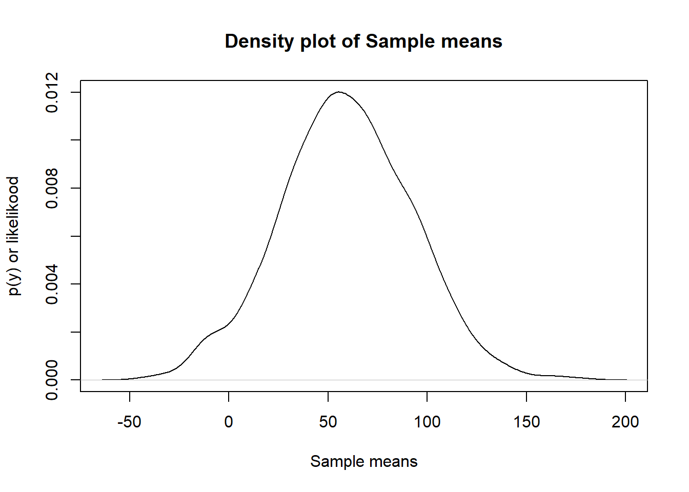
  • In this example I’ll generate 1000 “datasets” from a Gaussian process (normal distribution) with M = 60, sd = 100. Each data set will contain 10 observations.

  • After generating 1000 data sets, I’m estimating the mean of those simulated values.

  • Imagine you are asking the question how many minutes do you need to take a shower? to 10 participants, you then conduct the same study the next day with a different set of 10 participants every day until you get 1000 sets of 10 participants.

set.seed(563)
N <- 10

M <- 60

SD <- 100

## Number of data sets or replications
rep <- 1000

results <- list()

for(i in 1:rep){

results[[i]] <- mean(rnorm(n = N, mean = M, sd = SD))
}
plot(density(unlist(results)),
     xlab = "Sample means",
     ylab = "p(y) or likelikood",
     main = "Density plot of Sample means")

Central Limit Theorem (CLT) (cont.)

  • There is more beautiful qualities about the CLT. This rule applies to all distributions. When you increase the number of observations per sample, and the number of sample approach infinity. The sample of means will look Gaussian distributed (normally distributed).

  • Remember the Poisson distribution I mentioned some lectures behind?

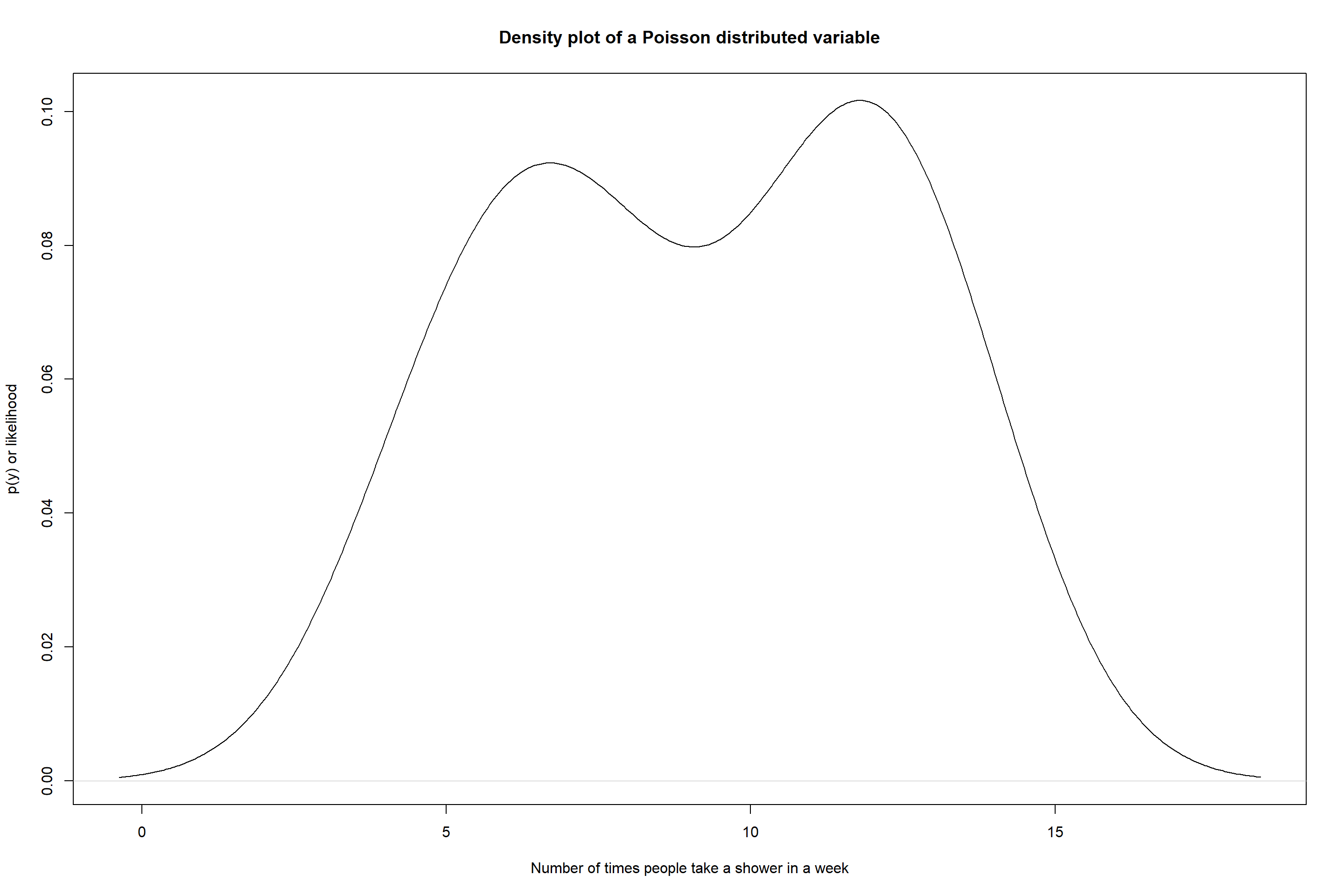
  • As you can see the Poisson distribution after generating 1 data set of 10 observations doesn’t look like a Gaussian process at all!

  • Can the sample of means from a Poisson process generate a pretty bell shape?

set.seed(563)
plot(density(rpois(n = 5,lambda = 8)),
     xlab = "Number of times people take a shower in a week",
     ylab = "p(y) or likelihood",
     main = "Density plot of a Poisson distributed variable")
set.seed(563)
plot(density(rpois(n = 10,lambda = 10)),
     xlab = "Number of times people take a shower in a week",
     ylab = "p(y) or likelihood",
     main = "Density plot of a Poisson distributed variable")

Central Limit Theorem (CLT) (cont.)

  • Let’s find out the answer by simulating 1000 data sets:
set.seed(563)
N <- 10

M <- 10

## Number of data sets or replications
rep <- 1000

results <- list()

for(i in 1:rep){

results[[i]] <- mean(rpois(n = N, lambda = M))
}
plot(density(unlist(results)),
     xlab = "Sample of means (Number of times people take a shower in a week)",
     ylab = "p(y) or likelihood",
     main = "Density plot of sample of means from a Poisson data process")

  • There is also something even prettier, the mean estimated with all the means, is actually close to the data generating process. It is lovely! This is a natural rule!
mean(unlist(results))
[1] 10.0076

Central Limit Theorem (CLT) (cont.)

  • We saw that the mean of sample means is close to the data generating process mean , and it doesn’t matter the type of distribution. However, take into account that there are probability distribution models that will require more than 800000000000 sampled means to approach the Gaussian shape. But eventually the distribution of all the means will look like a Gaussian distribution.

  • In simple terms, what does it mean? It means that the mean is an unbiased estimate on average it tends to be close to the “population” mean. This is why we like the mean as an estimate , and we use it to test hypothesis.

Standard Error

  • The CLT will be helpful to introduce the concept of standard error.

  • The Standard Error is a measure of how far is the mean of my sample from the true value in the data generating process.

  • The Standard Error in the context of multiple samples is the standard deviation of all sampled means.

  • We should go to another example:

Show the code
set.seed(563)
N <- 10

M <- 60

SD <- 100

## Number of data sets or replications
rep <- 1000

results <- list()

for(i in 1:rep){

results[[i]] <- mean(rnorm(n = N, mean = M, sd = SD))
}

cat("The Standard Deviation of 1000 sampled means is", sd(unlist(results)))
The Standard Deviation of 1000 sampled means is 33.25718
  • in this example if we estimate the standard deviation of our sample means we get sd = 33.2571782.

Standard Error (cont.)

  • In real life, you’ll never know the standard deviation of sample means, because this is a simulated example.

  • In real application you need to estimate how far your observed mean is from the true mean.

  • We can use this estimation \(\frac{\sigma}{\sqrt(n)}\) to approximate how far we are from the mean. In this formula \(\sigma\) is the standard deviation and \(n\) is the sample size.

  • The standard error decreases when we increase the sample size, let’s see another example:

Show the code
set.seed(563)

N <- seq(10, 10000, by = 10)

M <- 60

SD <- 100

results <- list()

for(i in 1:length(N)){

results[[i]] <- sd(rnorm(n = N[i], mean = M, sd = SD))/sqrt(N[i])
}
plot(x = N,
     y = results,
     type = "l",
     xlab = "Number of observations in each sample",
     ylab = "Standard error",
     main = "Line plot of Standard Error by sample size")

Important

In simple words: The standard error (SE) measures the distance from the true value in the data generating process.

More details about the Gaussian distribution

The 68–95–99.7 Rule for a Normal Distribution

  • There is an important concept in frequentist statistics called “confidence interval”

  • But before getting into details I need to explain a important property of the normal distribution.

  • The following rule applies for the normal distribution:

    • 68 \(\%\) of values will be between \(\mu\) - \(\sigma\) and \(\mu\) + \(\sigma\) .
    • 95 \(\%\) of values will be between \(\mu\) - \(2 \sigma\) and \(\mu\) + \(2 \sigma\).
    • 99.7 \(\%\) of values will be between \(\mu\) - \(3 \sigma\) and \(\mu\) + \(3 \sigma\)
  • We can see it by generating values from a Gaussian process:

library(ggplot2)

set.seed(3632)

generatedValues <- rnorm(200000, mean = 50, sd = 2)

### +-1 standard deviation form the mean

upper <- 50 + 2

lower <- 50 - 2

percent1sigma <- (sum(generatedValues <= upper & generatedValues >= lower)
/length(generatedValues))*100

### +-2 standard deviation form the mean

upper <- 50 + 2*2

lower <- 50 - 2*2

percent2sigma <- (sum(generatedValues <= upper & generatedValues >= lower)/length(generatedValues))*100

### +-3 standard deviation form the mean

upper <- 50 + 3*2

lower <- 50 - 3*2

percent3sigma <- (sum(generatedValues <= upper & generatedValues >= lower)/length(generatedValues))*100
  • 68.35 \(\%\) of observations are located at \(\pm 1 \sigma\) from the data generating process mean. That is true!

  • 95.45 \(\%\) of observations are located at \(\pm 2 \sigma\) from the data generating process mean. That is true!

  • 99.74 \(\%\) of observations are located at \(\pm 3 \sigma\) from the data generating process mean. That is true!

Allow me to use a metaphor

Westfall & Henning (2013):

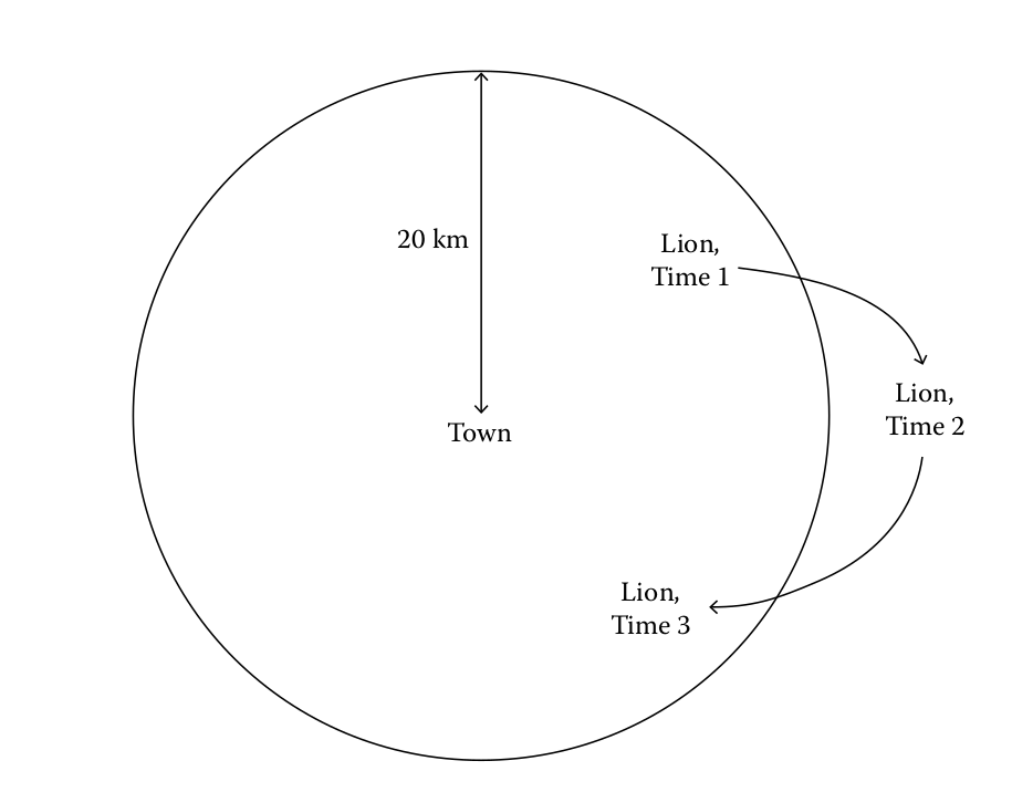
  • Imagine there is a lion or perhaps a coyote around your town. Every day the coyote moves around 20 km from the town, forming a circular perimeter. The town is right in the middle of the circle:

Allow me to use a metaphor (cont.)

  • As you can imagine the lion or coyote could move further from the town but it is always wondering around town chasing chickens or killing cows.

  • We could collect data, for instance, the distance every day from town, and see on average how far it is from town. We could also estimate the standard deviation (). This could be a good measure to see patterns, and be confident about the interval (circle) where the lion or coyote walks.

Allow me to use a metaphor (cont.)

  • Let’s imagine that the town is our data generating process mean value (). Also imagine that each time the lion or coyote walks around the town is an independent observed sample from the data generating process.

  • We need to find a way to be confident that our observed data is closed to \(\mu\) (“population mean”).

  • A few minutes ago we saw that according to the a Gaussian distribution, you’ll find 95 \(\%\) of the values around \(\pm 2 \sigma\) from the mean. However, in our simulated data we found out that in reality you’ll find more than 95 \(\%\). It was actually 95.45 \(\%\).

  • We’ll use this great property of the Gaussian distribution, but we will use \(\pm 1.96 \sigma\) instead of \(\pm 2 \sigma\). Why? because we want to be closer to exactly find 95\(%\) of the observations. This means, we want to be 95\(\%\) confident that we are close to \(\mu\), or the town following our example.

  • We will estimate the confidence interval by computing:

\[\begin{equation} \bar{x} \pm 1.96 \frac{\hat{\sigma}}{ \sqrt{n}} \end{equation}\]

Where,

\(\bar{x}\) is the estimated mean.
\(\hat{\sigma}\) is the estimated standard deviation.
\(1.96\) is the 97.5 percentile in the standard normal distribution (Gaussian).

Confidence Interval

Let’s compute the confidence interval by hand, we can use again the mean of the rumination score:

\[\begin{equation} 30.25 \pm 1.96 \Big (\frac{8.41}{\sqrt{205}} \Big ) \end{equation}\]

We need to estimate the mean first:

RumMean <- mean(na.omit(rum_scores$rumination))
RumMean
[1] 30.25854

Second, we need to estimate the standard deviation:

sd(na.omit(rum_scores$rumination))
[1] 8.406725

Now we can estimate the 95\(\%\) confidence interval:

upperCI <- 30.26+1.96*(8.41/sqrt(205))

lowerCI <- 30.26-1.96*(8.41/sqrt(205))

cat("The 95% confidence interval for the mean is:", 
        "upper-bound=",
        round(upperCI,2), 
        "lower-bound=",
          round(lowerCI,2))
The 95% confidence interval for the mean is: upper-bound= 31.41 lower-bound= 29.11

We can also estimate the confidence interval using the package rcompanion:

library(rcompanion)

Attaching package: 'rcompanion'
The following object is masked from 'package:effectsize':

    phi
groupwiseMean(rumination ~ 1,
              data   = rum_scores,
              conf   = 0.95,
              digits = 3,
              na.rm = TRUE)
   .id   n Mean Conf.level Trad.lower Trad.upper
1 <NA> 205 30.3       0.95       29.1       31.4
  • There is something to note here. What you are doing is just multipliying the standard error of the mean by 1.96. This value = 1.96 is called critical value.
##Standard error multiplied by 1.96
1.96*(8.41/sqrt(205))
[1] 1.151265
  • With the information above we could interpret our result as follows:

I am approximately 95\(\%\) confident that \(\mu\) is within 1.15 score points of the sample average 30.26.

Confidence Interval Intepretation

  • Many of the concepts studied up to this point come from a theory called “frequentist”.

  • The frequentist theory studies the probability in terms of long run events. In this approach we have to imagine that we repeat the same experiment or study several times. Only if we repeat the same study several times we’ll be able to create a confidence interval.

  • This is, of course theoretical. We are able to calculate confidence intervals with one sample. But, this interval is only an approximation.

  • The interpretation of the confidence interval demands to imagine that you repeat the same study \(n\) number of times. Hence the interpretation would be:

Since \(\mu\) will lie within the upper and lower limits of similarly constructed intervals for 95% of the repeated samples,my sample is likely to be one of those samples where \(\mu\) is within the upper and lower limits, and I am therefore 95% confident that \(\mu\) is between 29.1 and 31.4.

\[\begin{equation} 29.1 \le \mu \le 31.4 \end{equation}\]

Confidence Interval: multiple means

  • Let’s imagine a ask the same question: how many minutes do you need to take a shower?
  • We could ask the same question to 50 different people 100 000 times, and then estimate the mean. The frequentist theory says that the true value will be among the 95\(\%\) of the sampled means.

The final part … I promise

Repeated measures: compare two dependent means

  • We have only studied how to test the difference between independet groups.

  • However, many times we have research designs where we do a pre-test and a post-test.

  • For example, I could create an intervantion to treat depression. If I want to evaluate if there is an effect of the intervention I could measure the depression levels before the intervention, after that my participants will receive my new depression treatment. After they finish the intervention I measure again thei levels of depression.

  • In this example, we would like to see a lower score in depression after the intervention. We would also like to test if the mean difference between time 1 and time 2 is explained by chance alone.

Null hypothesis: \[\begin{equation} H_{0} = \mu_{posttest} = \mu_{pretest} \end{equation}\]

Repeated measures: compare two dependent means (cont.)

\[\begin{equation} t = \frac{\sum D}{\sqrt{\frac{n \sum D^2 - \big (\sum D \big )^2}{n-1}}} \end{equation}\]

\(D\) is the difference between each individual’s score from the first to the second time point.

\(\sum D\) is the sum of all the differences between groups of scores.

\(\sum D^2\) is the sum of the differences squared between groups of scores.

\(n\) is the number of pairs of observations.

Repeated measures: compare two dependent means (cont.)

  • We can test if the mean difference in life expectancy is explained by chance.

  • Let’s compare years 2019 and 2020:

lifeExpec <- read.csv("lifeExpect.csv")

t.test(lifeExpec$X2019, lifeExpec$X2020, paired = TRUE)

    Paired t-test

data:  lifeExpec$X2019 and lifeExpec$X2020
t = -0.19141, df = 243, p-value = 0.8484
alternative hypothesis: true mean difference is not equal to 0
95 percent confidence interval:
 -0.07583952  0.06240551
sample estimates:
mean difference 
   -0.006717005 

We failed to reject the null hypothesis according to the \(t\)-test for dependent means. How did we arrived to this conclusion?

Tip

Pay attention to the \(p-value\). Do you remember the null hypothesis in this case?

References

Cohen, J. (2013). Statistical Power Analysis for the Behavioral Sciences. Academic Press.
Westfall, P. H., & Henning, K. S. (2013). Understanding advanced statistical methods. CRC Press Boca Raton, FL, USA: