Correlation and Regression Models

Part 3: ANOVA and The General Linear Model

Esteban Montenegro-Montenegro, PhD

Psychology and Child Development

Why are we studying the regression model and other demons?

• Regression is only one member of the family of General Linear Model (GLM).

• The GLM covers models such as Analysis of Variance (ANOVA), Multivariate Analysis of Variance (MANOVA), Classical Regression Model (linear regression) and \(t\)-test.

• My aim was to introduce these topics as a generalization of GLM, or better said, as a family.

• There is a large theory related to these GLM models, but we don’t have time to discuss every detail. More advanced classes are necessary to explain particular details.

  graph TD
    A[GLM] --> B(ANOVA)
    A[GLM] --> C(MANOVA)
    A[GLM] --> D(t-test)
    A[GLM] --> E(Linear Regression)

Let’s make up time for ANOVA

• Analysis of Variance a.k.a ANOVA is a model that helps to analyze mean differences in multiple groups. It is actually very similar to the Classical Regression Model, that’s why I included ANOVA in the Classical Regression Model lecture.

• The ANOVA model tests the null hypothesis that all group means are equal. It could be represented like this:

\[\begin{equation} H_{0}: \mu_{1} = \mu_{2} = \mu_{3} \end{equation}\]

• This would be what we call an omnibus test, which means we are testing the overall effect of our independent variable on the dependent variable.

• As always, let’s understand this with an example:

Wage's mean, sd, and variance by Marital Status

maritl	M	SD	variance
1. Never Married	92.73	32.92	1083.73
2. Married	118.86	43.12	1859.38
3. Widowed	99.54	23.74	563.64
4. Divorced	103.16	33.80	1142.51
5. Separated	101.22	33.66	1133.22

• In the table above we can see the mean of wage by marital status, there are males who never married, married, widowed, divorced or separated. ANOVA will help us to answer the question:

Are the mean differences in wage by marital status explainable by chance alone?

• In this case ANOVA could tell us: Yes! there is a difference, but where?

• In this scenario, ANOVA will allow us to do pairwise comparisons , this means; we could compare the mean of divorced males versus the mean of married males, but also test all the combinations later on. This is called a post hoc analysis.

Let’s make up time for ANOVA (cont.)

• The ANOVA follows the logic of variance decomposition:

\[\begin{equation} outcome_{i} = (model) + error_{i} \end{equation}\]

• This means, that ANOVA accounts for the variances within your groups, and also calculates the variance that is explained by your MODEL. In fact, the Classical Regression Model does exactly the same thing.

• Remember: The line of best fit in regression is estimated adding the sum of square distances from the line. The line with the lowest sum of distances is the best line in regression.

• We are going to do something similar in ANOVA, it is called the Total Sum of Squares (\(SS_{T}\)), this calculation will give you the distance from the grand mean:

\[\begin{equation} SS_{T} = \sum^N_{i=1}(x_{i}-\bar{x}_{(grandMean)}) \end{equation}\]

• The term \(x_{i}\) is the score or value for each observation, and \(\bar{x}_{(grandMean)}\) is the overall mean.

Let’s make up time for ANOVA (cont.)

• We can continue with our example with wage \(\sim\) maritl.

• We can calculate the grand mean of wage:

WageGrandMean <- mean(Wage$wage)
WageGrandMean 

[1] 111.7036

• Now we could estimate \(SS_{t}\) in R:

sstData <- Wage |> select(wage, maritl) |> 
  mutate(SSt = (wage - mean(wage))^2)
  
sum(sstData$SSt)

[1] 5222086

The total \(SS\) is 5222086. This is the TOTAL variation within the data.

• We also need to estimate the Model Sum of Squares:

\[\begin{equation} SS_{M} = \sum^k_{n=1}n_{k}(\bar{x}_{k}-\bar{x}_{grandMean})^2 \end{equation}\]

• \(k\) represents each group, in simple words we are estimating the mean difference of each group from the overall mean. That’s the distance from the grand mean.

• We will need to estimate the residuals of the our model, the residuals is variance not explained by our ANOVA model. The estimation is:

Let’s make up time for ANOVA (cont.)

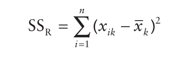
• In this estimation we calculate the difference of each observation from the group mean where the observation is located. So, for instance if Katie was in the divorced group, then we could compute: \(wage_{katie} - mean(wage_{divorced})\). This is an indicator of variation not explained by the model. This means, ANOVA does not explain what happens within each group’s variation, it accounts for the between group variation.

Time for examples !

Show the code

modelAnova <- aov(wage ~ maritl, data = Wage)
summary(modelAnova)

              Df  Sum Sq Mean Sq F value Pr(>F)    
maritl         4  363144   90786   55.96 <2e-16 ***
Residuals   2995 4858941    1622                   
---
Signif. codes:  0 '***' 0.001 '**' 0.01 '*' 0.05 '.' 0.1 ' ' 1

• The result showed that the difference is not explained by chance alone. But wait, this is an omnibus test. It just tell me that at least one mean is different.

Time for examples !

Show the code

  ggplot(data = Wage,aes(x=maritl, y=wage, fill=maritl)) +
    geom_boxplot() +
   stat_summary(fun="mean", color="red")+
    scale_fill_viridis(discrete = TRUE, alpha=0.6, option="A") +
    theme_classic()+
   theme(legend.position = "none")+
  labs(x= "Marital Status", y= "Wage", title = "Boxplot of Wage by Marital Status")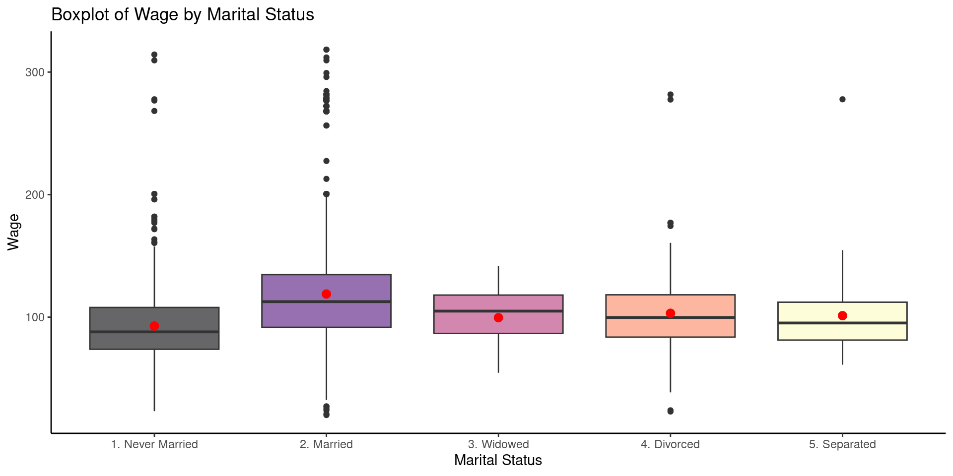

Time for examples !

• Let’s see the pairwise comparisons:

Show the code

pairTest <-TukeyHSD(modelAnova)




as.data.frame(lapply(pairTest, function(x) round(x,2))) %>%
  rename(meanDiff = maritl.diff,
          lower = maritl.lwr ,
         upper = maritl.upr ,
         pvalueAdj = maritl.p.adj
         ) %>%
 kbl(caption = "Pairwise Contrast") %>%
kable_classic_2("hover", full_width = T, 
                bootstrap_options = c("striped", "hover", "condensed", "responsive"))

Pairwise Contrast

	meanDiff	lower	upper	pvalueAdj
2. Married-1. Never Married	26.13	21.18	31.07	0.00
3. Widowed-1. Never Married	6.80	-18.78	32.39	0.95
4. Divorced-1. Never Married	10.42	1.60	19.25	0.01
5. Separated-1. Never Married	8.48	-6.96	23.92	0.56
3. Widowed-2. Married	-19.32	-44.66	6.02	0.23
4. Divorced-2. Married	-15.70	-23.77	-7.63	0.00
5. Separated-2. Married	-17.64	-32.66	-2.63	0.01
4. Divorced-3. Widowed	3.62	-22.75	29.99	1.00
5. Separated-3. Widowed	1.68	-27.58	30.93	1.00
5. Separated-4. Divorced	-1.94	-18.65	14.76	1.00

F ratio estimation

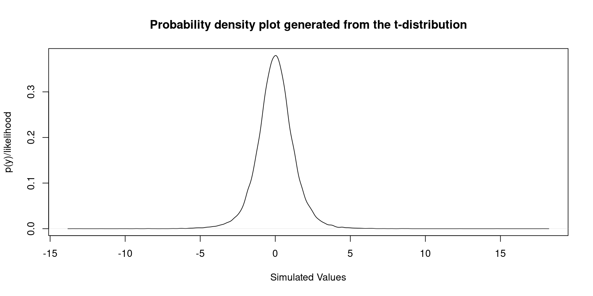
• In previous classes we studied the \(t\)-test. Hopefully, you remember the \(t\)-distribution:

Show the code

set.seed(234)

plot(density(rt(30000,5)),
     xlab = "Simulated Values",
     ylab = "p(y)/likelihood",
     main = "Probability density plot generated from the t-distribution")

F ratio estimation

• The t-distribution is used to find the probability of the estimated mean difference.

• In ANOVA we will use the F-distribution to find the probability of the estimated difference. In \(t\)-test we find only one mean difference, in ANOVA we will have several mean differences. The F-distribution will help us to test all the mean differences at the same time. That’s way we call omnibus test the first step in ANOVA.

• This distribution is a little bit peculiar. Because it requires degrees of freedom in the numerator and the denominator, we will see later how are we going to use these degrees of freedom in the context of the ANOVA.

F ratio estimation

Just another F distribution

Show the code

set.seed(234)
plot(density(rf(30000,5,10)),
     xlab = "Simulated Values",
     ylab = "Likelihood",
     main = "Probability density plot generated from the F-distribution")

F ratio estimation: let’s go to the point

• To estimate the F ratio we need first to estimate the Mean Squares based on the Sum of Squares.

• We previously saw the formula to estimate the \(SS_{R}\), which in simple words, the total variation due to external factors not controlled by the variables in the model. While \(SS_{M}\) is the total variation accounted by the ANOVA model. \[\begin{align} MS_{M} &= \frac{SS_{M}}{df_{M}}\\ MS_{R} &= \frac{SS_{R}}{df_{R}}\\ \end{align}\]

\(MS_{m}\) is the average amount of variation explained by the model (e.g., the systematic variation) , whereas \(MS_{R}\) is a gauge of the average amount of variation explained by extraneous variables (the unsystematic variation) (Field et al., 2012).

• The \(df\) in \(MS_{M}\) are estimated by subtracting 1 to the number of groups. In our example we have 5 groups, then we should do \(df = 5-1\). The degrees of freedom in \(MS_{R}\) are estimated by computing \(N-k\), where \(N\) is the sample size and \(k\) the number of groups. In our example would be \(df = 3000-5\).

• Let’s take a loot again at the ANOVA taht we estimated before:

Show the code

modelAnova <- aov(wage ~ maritl, data = Wage)
summary(modelAnova)

              Df  Sum Sq Mean Sq F value Pr(>F)    
maritl         4  363144   90786   55.96 <2e-16 ***
Residuals   2995 4858941    1622                   
---
Signif. codes:  0 '***' 0.001 '**' 0.01 '*' 0.05 '.' 0.1 ' ' 1

• Remember that we had 5 marital status groups, and the total sample is 3000 males. If you check the Df column in the table above you will see two numbers, the first one is 4 (\(5-1=4\)) , and the second number is 2995 (\(3000-5= 2995\)).

F ratio estimation: let’s go to the point

• After computing the Mean Squares and degrees of freedom, you’ll be able estimate the F ratio:

\[\begin{align} F &= \frac{MS_{M}}{MS_{R}}\\ &= \frac{90786}{1622}\\ &= 55.96\\ \end{align}\]

• The F in this case is a ratio of the variation explained by the model. If we conducted an experiment, we want a large F ratio because it would mean that we maximize the systematic variance explained by the experiment. Ideally, \(MS_{R}\) should be small.

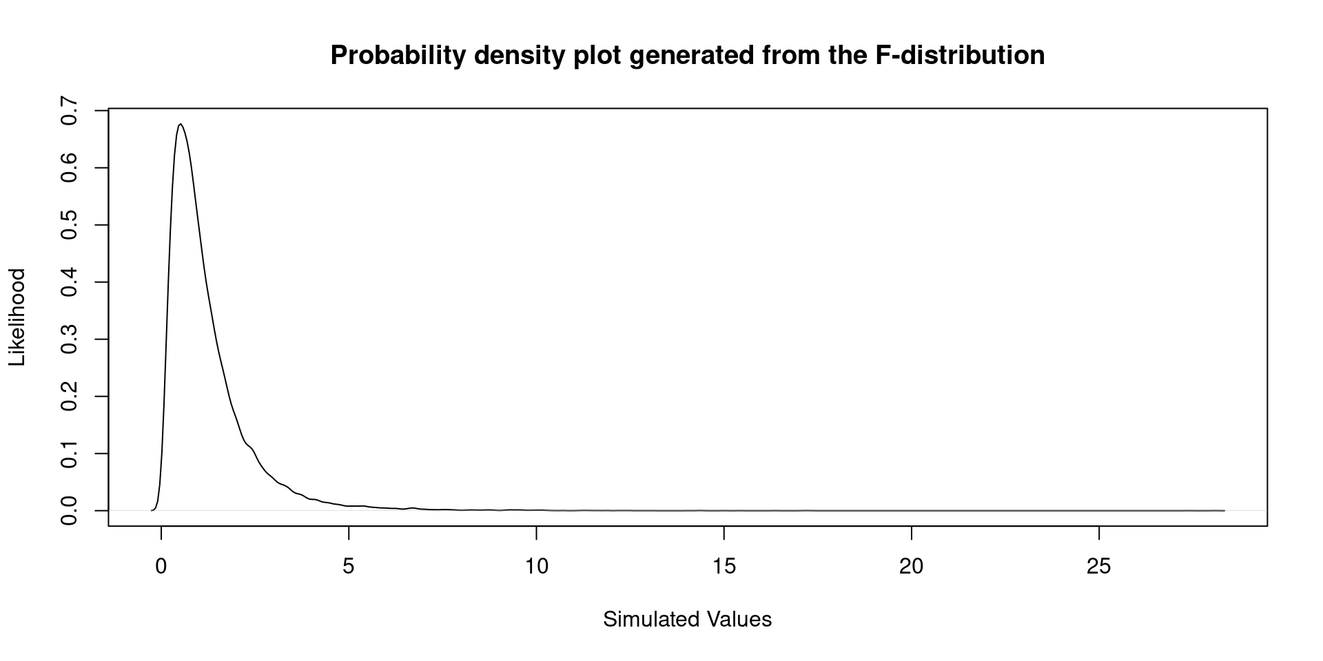
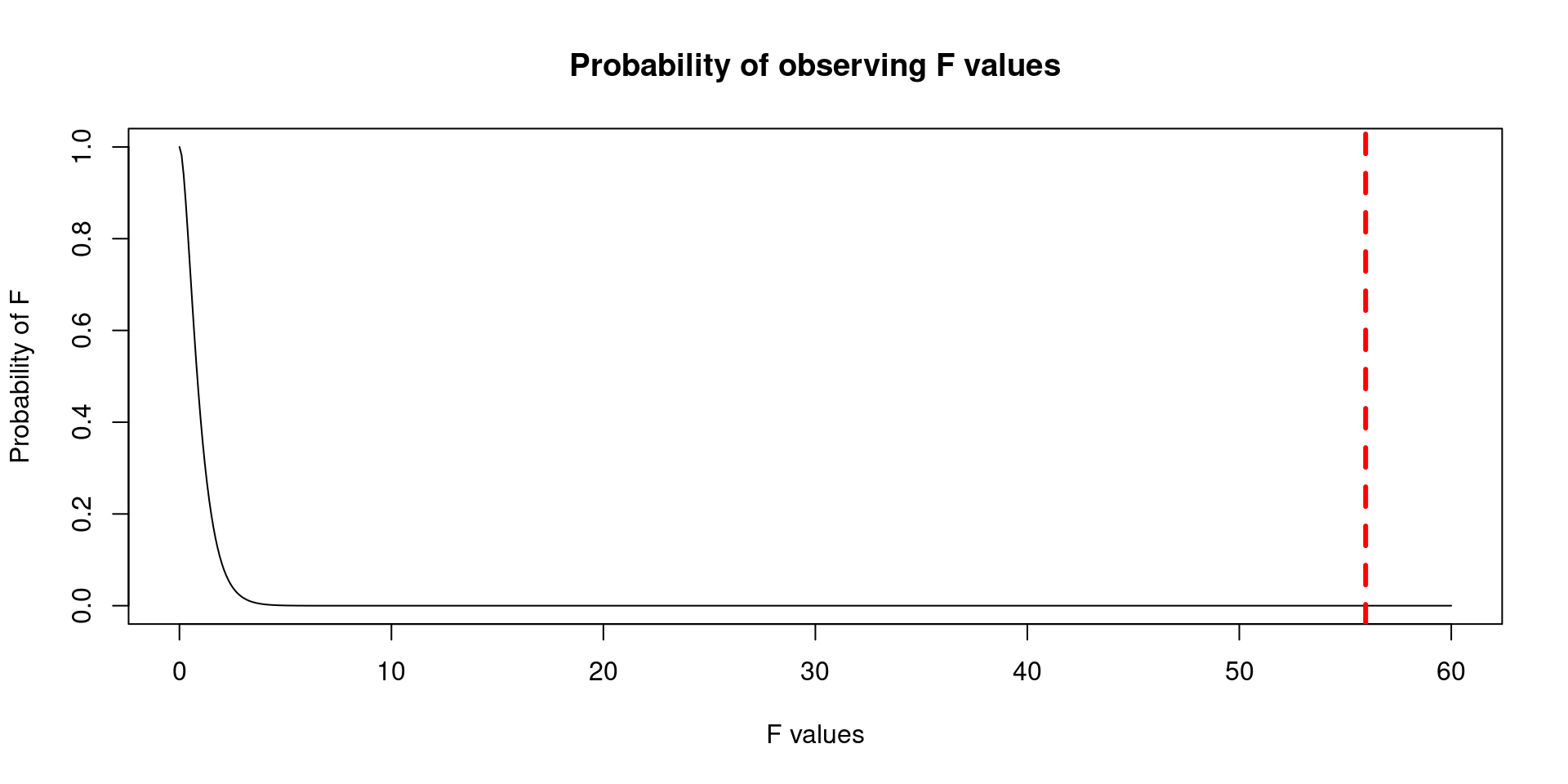
F ratio estimation: let’s go to the point

• The Cumulative Density Function of the F distribution will help us to estimate the probability of seeing a number as extreme as: 55.96. The red line corresponds to the location of 55.96.

Show the code

simValues <- seq(0,60,0.1)

values <-  pf(simValues, 
              df1 = 4, 
              df2 = 2995,
              lower.tail = FALSE)

plot(simValues, values, type = "l",
     xlab = "F values",
     ylab = "Probability of F",
     main = "Probability of observing F values")
abline(v = 55.96, col="red", lwd=3, lty=2)

Assumptions

ANOVA and Classical Regression Model

• One of the most important assumptions in ANOVA and Classical Regression Model is constant variance.

• When you estimate an ANOVA you could test this assumption using the Levene’s Test, the same test that we used to test the constant variance in \(t\)-test.

• The null hypothesis in the Levene’s test states: The variances of all groups are equal. If the test shows a \(p\)-value lower than 0.05, we reject the null hypothesis.

Show the code

library(car)
leveneTest(wage ~ maritl, data = Wage)

Levene's Test for Homogeneity of Variance (center = median)
        Df F value    Pr(>F)    
group    4  10.258 3.006e-08 ***
      2995                      
---
Signif. codes:  0 '***' 0.001 '**' 0.01 '*' 0.05 '.' 0.1 ' ' 1

• The result shows a \(p\)-value lower than 0.05, therefore we should reject the null hypothesis. The variances are not equal between groups.

Always remember!

ALL OF THE ASSUMPTIONS REFER TO THE DATA-GENERATING PROCESS. NONE OF THE ASSUMPTIONS REFER TO THE ACTUAL OBSERVED DATA (Westfall & Arias, 2020)

• In this case, we have a large sample size, this might cause a small p-value in the case of the Levene’s Test.

ANOVA and Classical Regression Model

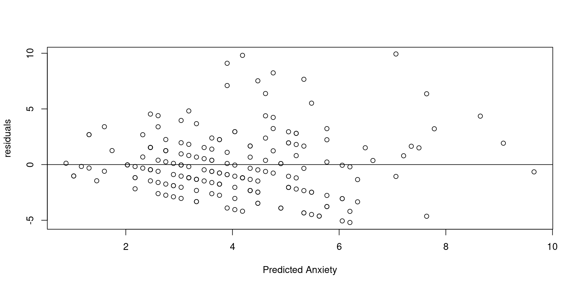
• In the context of regression we can plot the predicted values called \(\hat{y}\) (“yhat”), versus the residuals

Show the code

newWage <- Wage %>%  mutate(married = ifelse(maritl == "2. Married", 1,0),
                          widowed = ifelse(maritl== "3. Widowed", 1,0),
                          divorced = ifelse(maritl== "4. Divorced", 1,0),
                          separate = ifelse(maritl== "5. Separated", 1,0))



fitModel <- lm(wage ~ married  + widowed + divorced + separate, data = newWage)

y.hat = fitModel$fitted.values
resid = fitModel$residuals
plot(y.hat, resid,
     xlab = "Predicted wage",
     ylab = "residuals")
abline(h=0)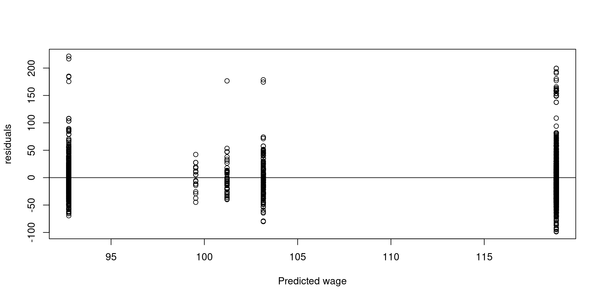

ANOVA and Classical Regression Model

• In the previous plot we can see more variability when the predicted wage is high. We can also see differences in variability in the lower income groups.

• We can plot similar information, but this time let’s use the absolute residuals:

Show the code

abs.resid = abs(resid)
plot(y.hat, abs.resid,
     xlab = "Predicted wage",
     ylab = "Absolute residuals",
     main = "Predicted wage by absolute residuals") 

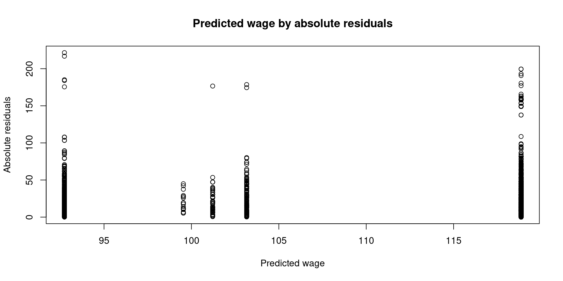
• Similar pattern, there is more variability in the groups where men earn more money. But is this bad for the linear model?

• It depends. We need to think if this is just part of the data generating process.

ANOVA and Classical Regression Model

• We can check the constant variance assumption in the context of a continuous predictor. This example only applies to Linear Regression, it won’t work with ANOVA because ANOVA only supports nominal predictors (groups).

Show the code

rum <- read.csv("ruminationClean.csv")

fitModel <- lm(anx ~ worry, data = rum)

y.hat = fitModel$fitted.values
resid = fitModel$residuals
plot(y.hat, resid,
     xlab = "Predicted Anxiety",
     ylab = "residuals")
abline(h=0)

ANOVA and Classical Regression Model

• Given that plots are sometimes difficult to interpret in this case, you might conduct another test called the Glejser test (Westfall & Arias, 2020).

• In this test we regress the absolute residuals on the predicted values. So, we are going to estimate a regression model to predict the residual, weird right?

• The short story is that we will get an slope, and if this slope is not explained by chance alone we will reject the constant variance assumption.

• Let’s test the constant variance assumption when we estimate anxiety \(\sim\) worry.

Show the code

### The target model
fitAnx <- lm(anx ~ worry, data = rum)
### get the residuals and predicted values
yhat <-  fitAnx$fitted.values ## predicted values
resi <- abs(fitAnx$residuals) ## residuals 

summary(lm(resi ~ yhat))

Call:
lm(formula = resi ~ yhat)

Residuals:
    Min      1Q  Median      3Q     Max 
-3.4731 -1.1677 -0.3061  0.8137  7.6189 

Coefficients:
            Estimate Std. Error t value Pr(>|t|)    
(Intercept)  0.71106    0.35353   2.011   0.0457 *  
yhat         0.35385    0.08094   4.372 2.01e-05 ***
---
Signif. codes:  0 '***' 0.001 '**' 0.01 '*' 0.05 '.' 0.1 ' ' 1

Residual standard error: 1.777 on 194 degrees of freedom
Multiple R-squared:  0.08968,   Adjusted R-squared:  0.08499 
F-statistic: 19.11 on 1 and 194 DF,  p-value: 2.009e-05

• In this case we cannot hold the assumption of homocedasticity (constant variance), because the estimated slope is not explained by chance alone (\(p < .001\)).

Classical Regression Model: normality assumption

• You can graphically evaluate if your model holds the assumption of normality. Remember that this assumption states that each conditional distribution \(p(y|x)\) is normally distributed.
• The best option is to plot the residuals of your model versus the quantiles of the normal distribution, this is called a QQ-Plot (quantile to quantile plot).

Classical Regression Model: normality assumption

Show the code

### The target model
fitAnx <- lm(anx ~ worry, data = rum)
### get the residuals and predicted values
res <- abs(fitAnx$residuals) ## residuals 
qqnorm(res)
qqline(res)

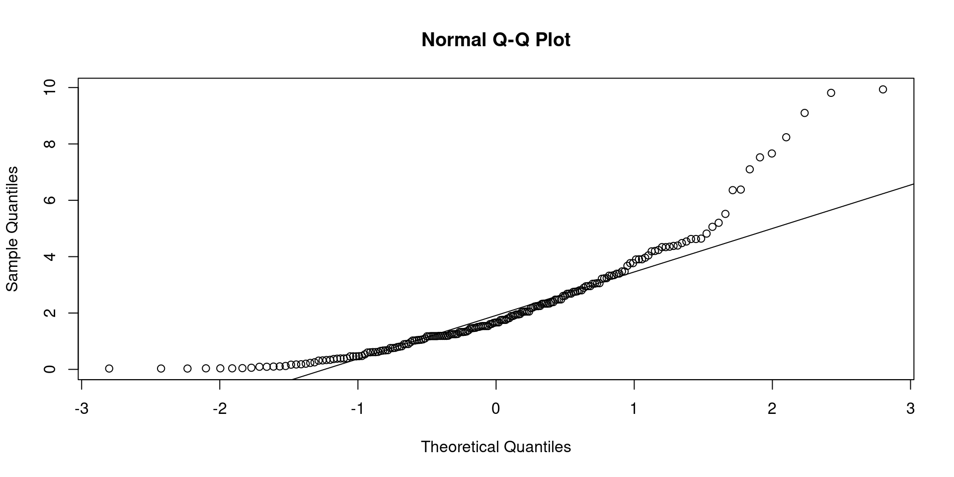
Classical Regression Model: normality assumption

• The qqplot can be sometimes difficult to read. We could perform a test called the Shapiro-Wilk test. In this test, the null hypothesis states “There is not deviation from the normal distribution”. A \(p\)-value less than .05 means that the model does not hold the assumption of conditional normality.

Show the code

shapiro.test(res)

    Shapiro-Wilk normality test

data:  res
W = 0.85861, p-value = 1.612e-12

• The Shapiro-Wilk test showed a p-value lower than .001, this means that the deviations of the residuals from the normal distribution are not explained by chance.

IMPORTANT!

The regression model and the General Linear Model does not assume that the outcome should come from a normally distributed process. That’s why the normality test is performed on the residuals of the model. The residuals are the product of the conditional relationship \(p(y|x)\). Don’t test the normality assumption on your dependent or outcome variable.

References

Field, A., Miles, J., & Field, Z. (2012). Discovering statistics using r. Sage publications.

Westfall, P. H., & Arias, A. L. (2020). Understanding regression analysis: A conditional distribution approach. Chapman; Hall/CRC.