Practice 2

What have you learned so far in R?

After completing the first practice, you should have learned these key concepts:

• R is an object-oriented programming language.
• R is free and open source, and you are able to install as many packages as you want for free.
• You learned the concept of “package”.
• You learned about data frames.

In this practice we will work with data frames , we will create new variables, and we will use extensively pipes along with the package tidyverse.

Good News!

In this practice you will be able to run R code straight from your web browser. Isn’t it awesome!

Let’s put a frame on those data points….

The data frame is one type of objects in R, and it is extremely useful to represent information as a data frame. This R object looks very similar to a spreadsheet in Excel, each column represents a variable, while each row represents an observation.

In this practice session we will wrangle the data set named ruminationToClean.csv. You may download the data set by Clicking Here. This is a dataset that was part of a large project that I conducted in Costa Rica in collaboration with a colleague and friend David Campos. Participants were high school students from the Central Valley in Costa Rica. The aim of this study was to explore the relationship between rumination and depression in teenagers. We added metacognitive beliefs to the study, but we will not talk about metacognition in this practice.

When I say wrangle I mean to manipulate the data set and clean the data. In real life, data sets are not perfectly clean. Many times we need to delete observations that are extreme cases (careless answers, mistakes, etc.), or sometimes we need to delete new variables. Additionally, we might need to compute new variables. We will cover all these topics in this practice using R.

The package tidyverse is your friend

If you run the following code, you’ll see the variable names in the data set ruminationToClean.csv:

I’m reading in the data file from my personal repository, fancy right?

Copy the code above to open ruminationToClean.csv in your R session.

As you can see, we have a large list of variables. We are using the function colnames() to get a list of column names, which in this case are research variables. Several of these variables could be dropped from the data set, others will need to be renamed.

Dropping variables

In this example we will use the function select() from the package tidyverse. Remember that you’ll need to call the package by running library(tidyverse).

What is happening here? You may have noticed that inside the function selection() I am adding the name of the variable I want to delete from the data set, and then I added a minus sign. When you add a minus sign before the name of the variable, the package will delete the variable that you list with a minus sign. You can do the same with several variables at the same time:

Now the variables, age, school, and grade are not longer in the dataset, if you don’t believe me click on RUN CODE.

Excercise 1 (15 points)

1. Download the data set ruminationToClean.csv then open the data file using ruminationRaw <- read.csv(file.choose()) or you may copy the code to open the data from the online repository. After opening the data in R, delete from the data set all the variables that start with th stem EATQ_R_.

Change variable names

In some occasions, the research variable was named wrongly or the name does not reflect the content of the variable. In the data set ruminationToClean.csv there are variables with names in Spanish, we can change them:

In this example, you can see that I’m using the function rename() from the package dplyr which is inside the package tidyverse. When you use rename() you’ll need to declare the new name first and then the old variable name that will be replaced.

Excercise 2 (15 points)

2. In psychological measurement it is common to implement questionnaires with Likert-response options. We typically sum the items corresponding to the latent variable or construct that we are measuring. For example in the ruminationToClean.csv the construct of “Rumination” is measured by the Children’s Response Styles Questionnaire (CRSQ), however the variable names are not self-explained. Your task is to change the name of the variables with stem CRSQ, the new variables should have the stem rumination_itemNumber. For example rename(rumination_1=CRSQ1). Remember to save the changes in a new object.

Compute a new variable

As always in programming languages, there are several ways to create a new research variable in a data frame. But, we will use the tidyverse method by using a function that actually works like a verb. The function mutate() will help use to create new variables.

I mentioned in Exercise 2 that psychology is a field that studies latent variables also known as hypothetical constructs, they have many names, but at the end we study variables that are implicit; we can measure them but we don’t see them. For example, we have studied variables such depression or rumination in this course, these are latent variables because you cannot capture depression or you don’t see it walking, however you are able to measure depression by asking about symptoms and thoughts.

Example of a latent variable

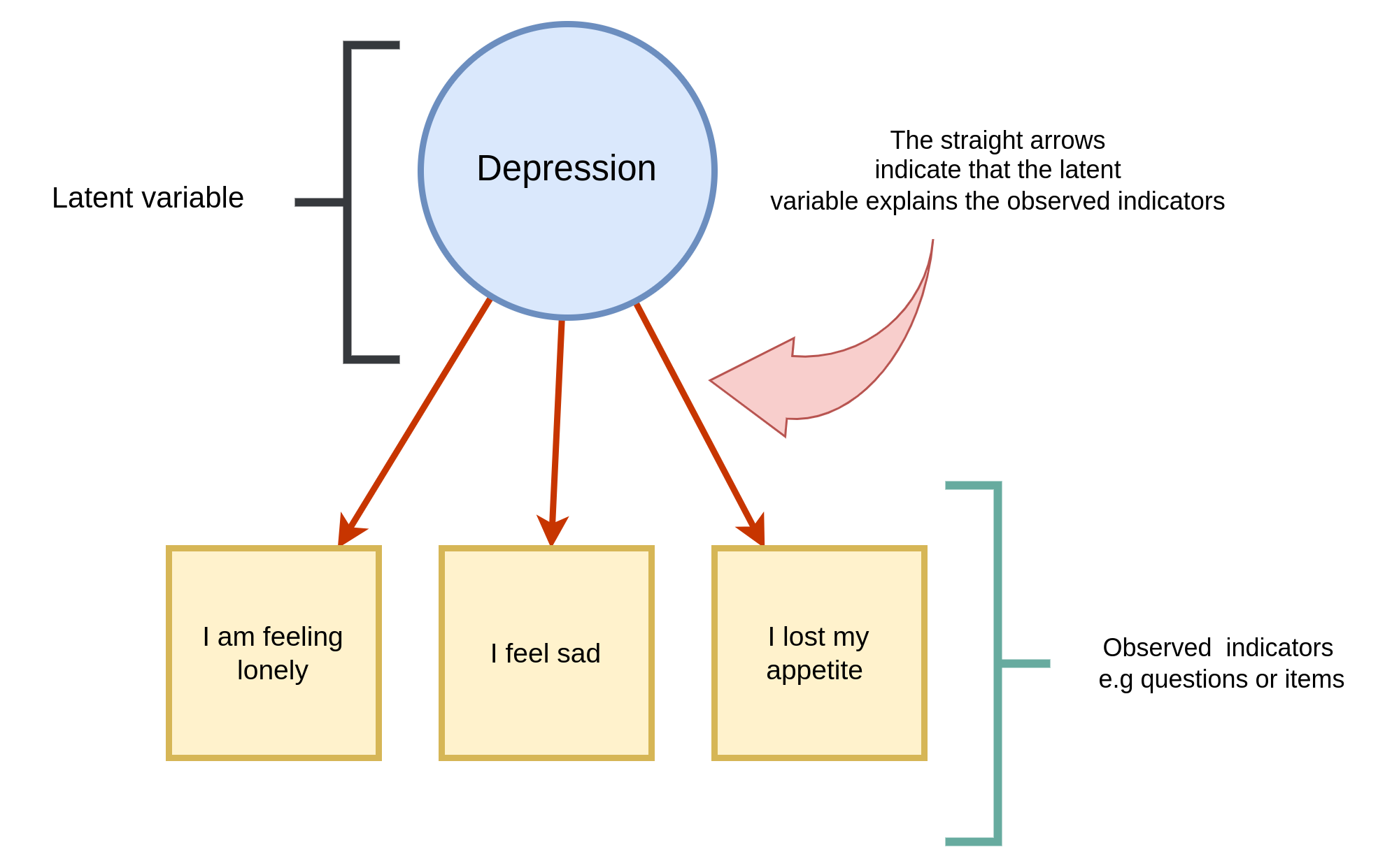
In the figure above you can see a representation of a latent variable. In psychology we often assume that the latent variable is the common factor underlying our questions, -in this example- questions related to depression.

When we analyze data that corresponds with latent variables we have two options:

1. We can create a Structural Equation Modeling (I won’t cover this topic).

2. We sum all the items to compute a total score. This total score will be our approximation to the latent variable. (Yes, this is covered in this practice).

I’ll show an example in the next chunk of R code:

In this example we are using the function mutate() to create a new column named depressionTotal, this new depressionTotal column will contain the depression total score for each participant. In this study we included the “Child’s Depression Inventory (CDI)”, that’s why the columns follow the stem “CDI”. You can see the new column in the next table:

ruminationRaw <- read.csv("ruminationToClean.csv", na.string = "99")
ruminationDepresionScore <- ruminationRaw |>
  mutate(
    depressionTotal = rowSums(across(starts_with("CDI")))
    )
ruminationDepresionScore |> select(starts_with("CDI"),  
                                   depressionTotal ) |>
  gt_preview()

	CDI1	CDI2	CDI3	CDI4	CDI5	CDI6	CDI7	CDI8	CDI9	CDI10	CDI11	CDI12	CDI13	CDI14	CDI15	CDI16	CDI17	CDI18	CDI19	CDI20	CDI21	CDI22	CDI23	CDI24	CDI25	CDI26	depressionTotal
1	0	2	0	0	0	0	0	1	0	0	1	0	1	1	1	1	1	1	1	0	0	1	1	1	1	0	15
2	0	0	1	1	0	0	0	1	0	0	1	0	2	0	1	0	2	1	1	0	0	1	2	1	0	0	15
3	0	1	0	0	0	1	0	0	1	0	0	0	0	0	0	0	0	0	1	0	0	0	0	0	0	0	4
4	0	1	0	0	0	0	0	0	0	0	0	1	1	0	0	0	1	1	0	0	0	0	0	1	0	0	6
5	0	1	0	1	0	1	0	0	1	1	0	2	1	1	0	1	1	2	0	1	0	0	1	1	1	0	17
6..211
212	0	0	0	0	0	0	0	0	0	1	0	0	0	1	0	0	0	1	0	0	0	1	0	1	0	0	5

Excercise 3 (15 points)

3. In the data set ruminationToClean.csv you’ll find seven columns with the stem “DASS”. These columns correspond to the instrument named: Depression, Anxiety, and Stress Scale (DASS). This is an scale that measures three latent variables at the same time, but only the anxiety items were added in this study.

Your task is to change the name of the “DASS” items, you should think a more informative name for these items in the data frame. After that, you will have to compute the total score of anxiety for each participant in the data frame.

Let’s cleanse this data set

It is always satisfactory to clean a data set and then see the final product, but so far we have cleaned these data in small steps. I’ll clean the data set in one step. In this example I will delete unnecessary columns (a.k.a research variables), and I will translate the variables to English when necessary:

Excercise 4 (15 points)

4. Describe the steps taken in the R code above.

Examine your data

In this second part we will create several plots to examine and explore our data. But first we’ll need to compute total scores again, because after all, the main point is to make conclusions about our latent variables (a.k.a latent factors).

We have now three total scores corresponding to three different latent factors: depression, anxiety, and depression. We are in a good place to explore the data. It is healthy to start looking at histograms because they are now continuous variables:

We can see in the histogram that low values are more frequent. This is expected because all the participants are healthy teenagers without any history of psychopathology. Also, pay attention that we are using the function hist() in R.

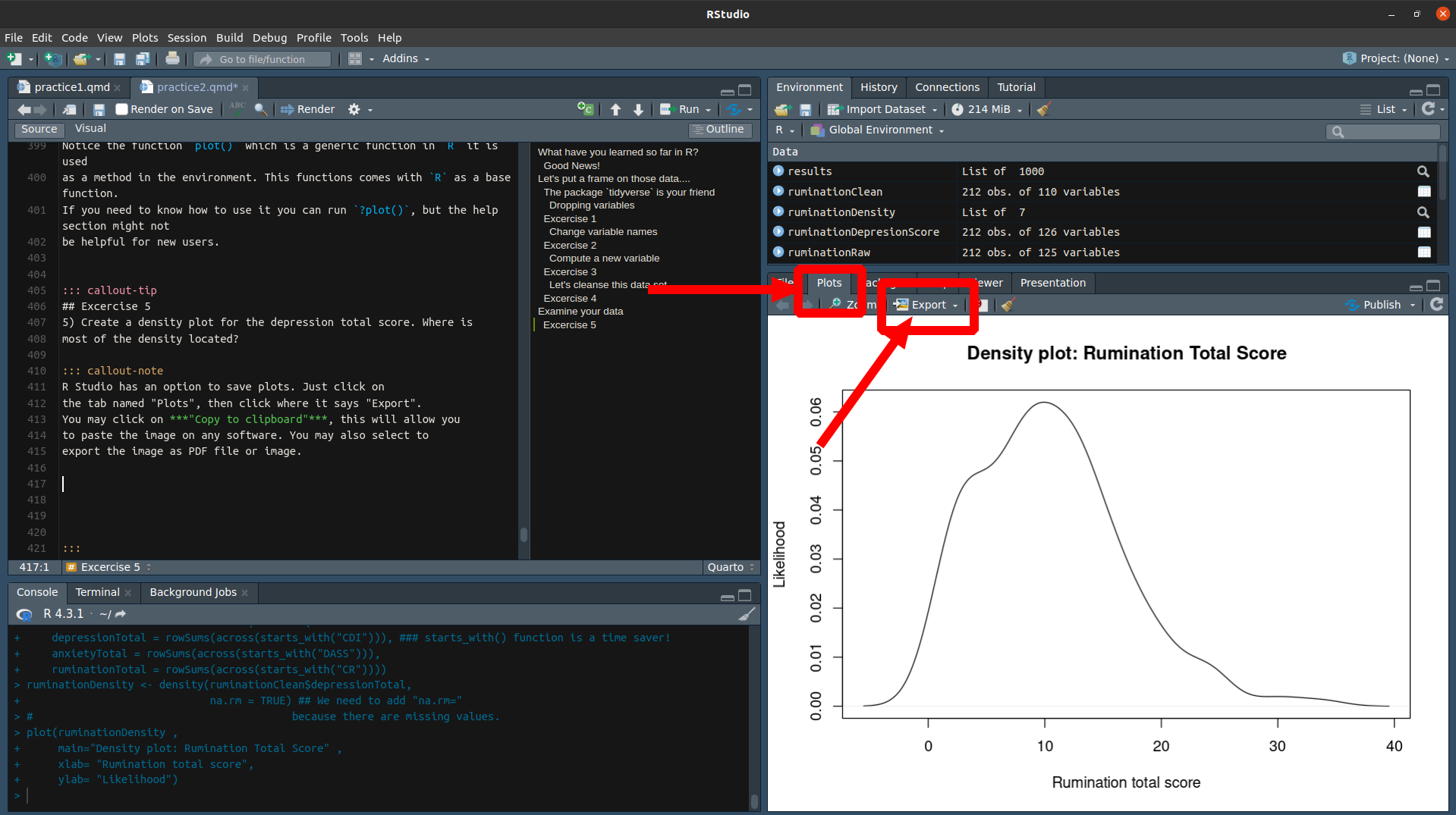
We can also generate a density plot to have an idea of the observed shape:

Notice the function plot() which is a generic function in R it is used as a method in the environment. This functions comes with R as a base function. If you need to know how to use it you can run ?plot(), but the help section might not be helpful for new users. Additionally, pay attention on how you can change the labels in your plot.

Excercise 5 (30 points)

5. Create a density plot for the depression total score. Where is most of the density located?

Note

R Studio has an option to save plots. Just click on the tab named “Plots”, then click where it says “Export”. You may click on “Copy to clipboard”, this will allow you to paste the image on any software. You may also select to export the image as PDF file or image.

Option to save generated plots

Box plots are also useful to understand our data better, you may revisit the box plot’s anatomy in this website: link.

We can see the next example (Click on Run Code):

Excercise 6 (15 points)

6. Can you tell which group in the box plot has the highest median in rumination? What else can you see in the box plot?

Special topics in R

You may remember that I mentioned multiple times how R objects have particular characteristics. This is time to study a few of these characteristics.

We will cover special characteristics of missing values.

Missing data without missing the point….

In scientific research is always problematic when a participant forgets to answer a question, it is more problematic when a participant drops from our study when conducting a longitudinal study. These scenarios are a nightmare for researchers.

I will not demonstrate all the possible missing data treatments, but I will show you how R deals naturally with missing values, and how you can code your missing values in your data set.

You have an NA on your face

In R you will see that missing values are flagged with NA. In the rumination data set you will see NA values like the ones on red:

ruminationRaw |> 
  select(starts_with("PSWQC")) |> 
  gt_preview()|>
   data_color(
    columns = c(PSWQC_7, PSWQC_7r, PSWQC_9r),
    method = "numeric",
    palette = "grey",
    domain = c(0, 50),
    na_color = "red"
  )

	PSWQC_1	PSWQC_2	PSWQC_3	PSWQC_4	PSWQC_5	PSWQC_6	PSWQC_7	PSWQC_8	PSWQC_9	PSWQC_10	PSWQC_11	PSWQC_12	PSWQC_13	PSWQC_14	PSWQC_2r	PSWQC_7r	PSWQC_9r
1	2	1	2	3	2	1	1	1	1	2	3	1	0	3	12	2	2
2	1	0	2	1	3	1	0	0	0	1	1	1	0	3	4	12	3
3	0	0	3	3	3	3	0	3	0	3	3	3	3	3	24	3	3
4	1	1	1	1	1	1	NA	0	1	0	1	0	1	0	2	NA	NA
5	2	0	2	2	3	1	2	0	0	1	2	2	1	2	3	1	3
6..211
212	0	1	1	1	0	0	3	0	2	0	3	0	0	0	3	2	0

NA stands for “non-applicable” and it became the flag for missing values. It is already built-in with R. You could change this flag but that is not necessary.

You can add NA to any vector, list, or data frame, see the following example:

vectorNames <- c("Adrian", "Marco", "Sofia")
### Let's add a missing value
vectorNames[3] <- NA 
vectorNames

[1] "Adrian" "Marco"  NA      

In this example, I added NA in the third position, but of course you could add NA anywhere in a vector.

In R there are functions that will return a logical value. Logical data contains only TRUE or FALSE, or 0 or 1. We can see an example with our vector with missing values.

## is.na() function will be your friend
is.na(vectorNames)

[1] FALSE FALSE  TRUE

The function is.na() returned a new logical vector flagging TRUE where there is a missing value. In this example is the third element.

Excercise 7 (15 points)

7. Search on Internet how to write a command where we ask the opposite: “show me TRUE when the value is not missing” .

HINT: You may need the exclamation character.

Add NA when you read in data

When you are opening a data set in R you will always need to specify how you flagged or coded your missing information. For example, it is usual to observe the number “-99” when values are missing, it is also possible to use “99” like I did in my rumination study. The main point is to select a number that is not possible to be found in your data set. In the rumination data set, it is impossible to expect a value “99” as a valid score. Because all the scores range from zero to maximum 20. Observe what I did at the beginning of this practice:

dataLink <- "https://raw.githubusercontent.com/blackhill86/mm2/main/dataSets/ruminationToClean.csv"

ruminationRaw <- read.csv(url(dataLink ),
                          na.strings = "99") 

In the code above, I’m adding the argument na.string = "99" to the function read.csv(). I did it because I flagged my missing values with “99”.

Important!!

If your external file has empty cells, R will interpret empty cells as missing values NA.

Usual questions when you are learning data coding and stats

Can I replace missing values with zeros?

The straight answers is a well rounded and pretty NO!!!

A zero is not equivalent to missing value. When you collect data you need to think first how you will code your missing values.

Can I replace missing values with the mean?

The short answer is NO! But, I’ll give you a longer answer, I’m a professor after all, it is my weakness!

When you replace a missing value with the mean value of an observed distribution, you are doing mean imputation. Long time ago, when computers where not fast, it was faster to replace missing values using the mean, it was easy, and it didn’t require to have a computer. But, nowadays it is not necessary to follow this practice anymore. However, there are still researchers using this replacement method.

If you assume that the estimated mean is a good representation of your missing value you will inflate your distribution with values close to the observed mean, which is wrong. Let’s see an example.

In this example, I will simulate a regression model. we haven’t covered the theory related to regression but I ebelieve I can explain some details in simple words.

The data-generating process will be the following:

\[Y \sim \alpha + \beta_{1}X_{1} + \beta_{2}X_{2} + \beta_{3}X_{3} + \epsilon \tag{1}\] You may have noticed that all “X” are uppercase and “Y” is uppercase. This means that any outcome \(Y\) will be predicted by \(X_{1}\), \(X_{2}\), and \(X_{2}\). This is the model that generates the data. However, given that this is a simulation we can be in control of the process, we can assume that the “population” model looks like this:

\[Y \sim 1 + (0.2)X_{1} + (0.3)X_{2} + (0.4)X_{2} + \epsilon \tag{2}\]

Let’s create 2000 data sets with this model in each data set there will be 100 observations.

library(MASS)
library(purrr)
library(patchwork)
library(ggplot2)

#### Let's simulate some data
set.seed(1236)

generateCompleteData <- function(n){

library(MASS)
MX <- rep(0, 3)
SX <- matrix(1, 3, 3)
SX[1, 2] <- SX[2, 1] <- 0.5
SX[1, 3] <- SX[3, 1] <- 0.2
SX[2, 3] <- SX[3, 2] <- 0.3
X <- mvrnorm(n, MX, SX)
e <- rnorm(n, 0, sqrt(0.546))
y <- 1 + 0.2 * X[,1] + 0.3 * X[,2] + 0.4 * X[,3] + e

reg <- lm(y ~ X[,1] +  X[,2] + X[,3])

dataReg <- data.frame(inter = reg$coefficients[[1]],
                      x1 = reg$coefficients[2],
                      x2 = reg$coefficients[3],
                      x3 = reg$coefficients[4])
                    

return(dataReg)

}

### Multiple models

allModels <- map_df(1:2000, ~generateCompleteData(100))


interPlot <- ggplot(allModels, aes(x=inter)) + 
  geom_density(fill = "blue",alpha = 0.2 )+
  geom_vline(xintercept = round(mean(allModels$inter),2), color = "red")+
  annotate("text", 
           x = 0.85, 
           y = 5, 
           label = paste0("M=", round(mean(allModels$inter),2)," ", 
                          "SD=", round(sd(allModels$inter),2)),
           color = "red")+
  xlab("2000 intercepts")+
  ylab("Likelihood")+
  theme_classic()
  
x1Plot <- ggplot(allModels, aes(x=x1)) + 
  geom_density(fill = "blue",alpha = 0.2 )+
  geom_vline(xintercept = round(mean(allModels$x1),2), color = "red")+
  annotate("text", 
           x = 0.4, 
           y = 5, 
           label = paste0("M=", round(mean(allModels$x1),2)," ", 
                          "SD=", round(sd(allModels$x1),2)),
           color = "red")+
  xlab("Estimated slopes X1")+
  ylab("Likelihood")+
  theme_classic()


x2Plot <- ggplot(allModels, aes(x=x2)) + 
  geom_density(fill = "blue",alpha = 0.2 )+
  geom_vline(xintercept = round(mean(allModels$x2),2), color = "red")+
  annotate("text", 
           x = 0.5, 
           y = 5, 
           label = paste0("M=", round(mean(allModels$x2),2)," ", 
                          "SD=", round(sd(allModels$x2),2)),
           color = "red")+
  xlab("Estimated slopes X2")+
  ylab("Likelihood")+
  theme_classic()

x3Plot <- ggplot(allModels, aes(x=x3)) + 
  geom_density(fill = "blue",alpha = 0.2 )+
  geom_vline(xintercept = round(mean(allModels$x3),2), color = "red")+
  annotate("text", 
           x = 0.6, 
           y = 5, 
           label = paste0("M=", round(mean(allModels$x3),2)," ", 
                          "SD=", round(sd(allModels$x3),2)),
           color = "red")+
  xlab("Estimated slopes X3")+
  ylab("Likelihood")+
  theme_classic()

interPlot  + x1Plot +
x2Plot + x3Plot  

Simulated values with complet information

As expected, the density plots for our parameters showed that after replicating the same study 2000 times the mean value is exactly at the target. The target are the values that we set in our “population” model in equation Equation 2.

In the next step, I will impose missing values on the data generated, we will see what happens when we replace the values with the mean of the observed distribution.

library(simsem)

set.seed(1236)

generateIncompleteData <- function(n){

library(MASS)
library(simsem)  
  
MX <- rep(0, 3)
SX <- matrix(1, 3, 3)
SX[1, 2] <- SX[2, 1] <- 0.5
SX[1, 3] <- SX[3, 1] <- 0.2
SX[2, 3] <- SX[3, 2] <- 0.3
X <- mvrnorm(n, MX, SX)
e <- rnorm(n, 0, sqrt(0.546))
y <- 1 + 0.2 * X[,1] + 0.3 * X[,2] + 0.4 * X[,3] + e


dataGen <- data.frame(outcome = y,
                      x1 = X[,1],
                      x2 = X[,2],
                      x3 = X[,3]) 


datMis <- imposeMissing(dataGen, 
                         pmMAR = .15, cov="x3")

meanOutcome <- mean(datMis$outcome, na.rm = TRUE)
meanX1 <- mean(datMis$x1, na.rm = TRUE)
meanX2 <- mean(datMis$x2, na.rm = TRUE)

datMis$outcome[is.na(datMis$outcome)] <- meanOutcome 
datMis$x1[is.na(datMis$x1)] <- meanX1
datMis$x2[is.na(datMis$x2)] <- meanX2


reg <- lm(outcome ~ x1 + x2 + x3, data = datMis)

dataReg <- data.frame(inter = reg$coefficients[[1]],
                      x1 = reg$coefficients[2],
                      x2 = reg$coefficients[3],
                      x3 = reg$coefficients[4])
                    

return(dataReg)

}

allModelsMissing <- map_df(1:2000, ~generateIncompleteData(100))


interPlotMissing <- ggplot(allModelsMissing, aes(x=inter)) + 
  geom_density(fill = "blue",alpha = 0.2 )+
  geom_vline(xintercept = round(mean(allModelsMissing$inter),2), color = "red")+
  geom_vline(xintercept = 1, color = "blue")+
  annotate("text", 
           x = 0.85, 
           y = 5, 
           label = paste0("M=", round(mean(allModelsMissing$inter),2)," ", 
                          "SD=", round(sd(allModelsMissing$inter),2)),
           color = "red")+
  xlab("2000 intercepts")+
  ylab("Likelihood")+
  theme_classic()
  
x1PlotMissing <- ggplot(allModelsMissing, aes(x=x1)) + 
  geom_density(fill = "blue",alpha = 0.2 )+
  geom_vline(xintercept = round(mean(allModelsMissing$x1),2), color = "red")+
  geom_vline(xintercept = 0.2, color = "blue")+
  annotate("text", 
           x = 0.4, 
           y = 5, 
           label = paste0("M=", round(mean(allModelsMissing$x1),2)," ", 
                          "SD=", round(sd(allModelsMissing$x1),2)),
           color = "red")+
  xlab("Estimated slopes X1")+
  ylab("Likelihood")+
  theme_classic()


x2PlotMissing <- ggplot(allModelsMissing, aes(x=x2)) + 
  geom_density(fill = "blue",alpha = 0.2 )+
  geom_vline(xintercept = round(mean(allModelsMissing$x2),2), color = "red")+
  geom_vline(xintercept = 0.3, color = "blue")+
  annotate("text", 
           x = 0.5, 
           y = 5, 
           label = paste0("M=", round(mean(allModelsMissing$x2),2)," ", 
                          "SD=", round(sd(allModelsMissing$x2),2)),
           color = "red")+
  xlab("Estimated slopes X2")+
  ylab("Likelihood")+
  theme_classic()

x3PlotMissing <- ggplot(allModelsMissing, aes(x=x3)) + 
  geom_density(fill = "blue",alpha = 0.2 )+
  geom_vline(xintercept = round(mean(allModelsMissing$x3),2), color = "red")+
  geom_vline(xintercept = 0.4, color = "blue")+
  annotate("text", 
           x = 0.5, 
           y = 5, 
           label = paste0("M=", round(mean(allModelsMissing$x3),2)," ", 
                          "SD=", round(sd(allModelsMissing$x3),2)),
           color = "red")+
  xlab("Estimated slopes X3")+
  ylab("Likelihood")+
  theme_classic()

interPlotMissing  + x1PlotMissing +
x2PlotMissing + x3PlotMissing  

Simulated values after replacing missing data with the mean

This time the estimated mean of all the slopes and intercepts moved a little bit far from the target, the blue line is our target value, and the red line is the estimated mean after replacing missing values with mean. You may think, that this is not a big deviation but in more complicated models with more parameters, this deviation from the target can cause harm to the point that you are not sure about your results. This is one reason why we don’t replace missing values with the mean.

So, what should we do instead of using mean imputation?

You may estimate your models using listwise deletion, this method deletes any case that contains a missing value. This is actually the default behavior in many software. We can study an example:

In this example I’m generating a vector with random numbers, and then I’m esimating the mean:

### Let's create a vector with complete values
vectorComplete <- c(123,56,96,89,59)
### We can estimate the mean:
mean(vectorComplete)

[1] 84.6

The mean is M=84.6, but notice what happens when there is a missing value:

### Let's delete some values to investigate what happens

vectorMissing <- c(123,56,NA,89,59)
mean(vectorMissing)

[1] NA

Now the mean() function returns nothing, it returns NA, why? Because you cannot compute anything if there is an empty slot. You need to delete the observation that is missing and then compute the mean again. This is what is called listwise deletion. You can enable listwise deletion by adding the argument na.rm = TRUE to the mean() function:

### Let's delete some values to investigate what happens

vectorMissing <- c(123,56,NA,89,59)
mean(vectorMissing, na.rm = TRUE)

[1] 81.75

Excercise 8 (15 point)

8. Fix the following code when estimating the correlation:

### mtcars is a data set already built into R
dataCars <- mtcars

### I'm imposing missing value on values located at 6,7,8,9
dataCars$mpg[c(6,7,8,9)] <- NA 

cor(dataCars$mpg, dataCars$hp) ### This function cor() should give us a estimated correlation, what is wrong?

[1] NA

HINT: You may check the help provided for the function cor() by typing ?cor on your R console. Or search on Internet.

Final note (I promise it is the end)

The best strategy to deal with missing values is something call multiple imputation, it is a statistical model that generates multiple data sets with possible values. Although, this is a topic for a second course in statistics.

---