library(parameters)
library(gtsummary)

url <- "https://raw.githubusercontent.com/blackhill86/mm2/refs/heads/main/dataSets/ouesData.csv"

ouesData <- read.csv(url)Introduction
In this section we will play with the dataset that I called “OUESdata”. This was part of a project I helped to develop, and later I tried to publish an article, well… the article was never publish but it is a good data set for teaching.
What is the story behind the the data set ouesData?
As you might imagine, you will need to read a story about this data set. This was a project conducted by several researchers from Costa Rica and United States.
The aim was to collect information to understand why Costa Ricans have a longer life compare to most people in United States. I was part of the team, I helped collecting some variables, and at the end I had a humble role as a data analyst.
This ouesData is only a small portion of variables collected in the context of the project named Epidemiology and Development of Alzheimer’s Disease (EDAD). All participants are aging adults older than 60 years old.
The variables included in this data set are:
Stroop_color: The first part of the Stroop test.
Trail_A,Trail_A_errors, Trail_B, Trail_B_errors: Trail Making Test
OUES: Oxygen uptake efficiency slope
VO2peak: Oxygen capacity
WAISR_block: WAIS block design.
WAISR_DSS: Digit Symbol Substitution Test
Six_min_walk: Distance walked in yards. Not useful for model selection.
HR_max: Maximum heart rate during the 6 minutes walk.
HR_pre: Heart rate before the 6 minutes walk.
Female: gender, 1= Female, 0 = Male.
delayedLM: delayed logic memory.
SRT_free_recall_trial1, SRT_free_recall_trial2, and SRT_free_recall_trial3: Buschke Selective Reminding Test (SRT) is when a participant is asked to recall as many words as possible from a list of words without a cue.
logicMemory: logic memory, how much detail can the participant remember after hearing a story.
fatTotal: Total body fat.
Country: 1= Kansas, 0= Costa Rica.
BMI: Body Mass Index.
SRT_total: Total score for the Buschke Selective Reminding Test (SRT).
Let’s open the data in R
For the the next task, you will need to open the data in R, you may use the following code:
TipInstall the following packages
In this assigment you will have to install the packages parameters and gtsummary. You can install it by running ONLY once:
install.packages(c("gtsumamry", "parameters"), dependencies = TRUE)You may also go to packages --> install --> type the name of the package
Correlations will help to know more
This is a new data set, and most likely you don’t know much about the theory behind the data. This makes more important to explore correlations between the variables in this dataset. We should focus on the relationship of *** cognition with cardiovascular fitness ***.
You will need the next list of variables, this list will help you to select the variables that you would like to correlate:
vars <- c("Stroop_color",
"Trail_A",
"Trail_A_errors",
"Trail_B",
"Trail_B_errors",
"OUES",
"VO2peak",
"WAISR_block",
"WAISR_DSS"   ,
"Six_min_walk" ,
"HR_max",
"HR_pre" ,
"Age"  ,
"Female",
"educa"  ,
"PeakRER" ,
"PHY.WeightKG.2",
"PHY.HeightCM.1" ,
"delayedLM"    ,
"SRT_free_recall_trial1" ,
"SRT_free_recall_trial2" ,
"SRT_free_recall_trial3",
"logicMemory"     ,
"RER"    ,
"fatTotal",
"BMI"      ,
"SRT_total" )
The following code will help you to estimate the correlation matrix, but this correlation matrix is large, you can reduce the number of correlated variables by changing the vector vars.
round(cor(ouesData[vars], use = "pairwise.complete.obs"),2)
Important1.Question:
Change the code presented above, estimate a smaller correlation matrix. You may reduce the number of variables based on theoretical assumptions, based on correlation values, or you could prioritize especific correlations.
Building a model
We usually need theory to start building a model, I know you might not be familiar with oxygen levels when practicing physical activity, but I will estimate a possible model, in the next section it will be your turn to find the best model.
In the following model, OUES will be a predictor in addition to other covariables.
The model will look like this:
\(WAISR_block = OUES + VO2peak + WAISR_DSS + HR_max\)
Dropping missing values
Before fitting any model, it is better to drop participants with missing values. Why? Well, we can use a metaphor for this, in this case let’s think about a russian doll:

When we are selecting and comparing models, each model is like a russian doll inside another rusian doll. You may remember when I showed you that you could fit a null model that estimates only the mean of your outcome like this:
formula <- depression ~ 1 In the model above we don’t have any predictor or independent variable, what we have is only a model that estimates the mean of depression.
In a more formal representation we are estimating a model like this:
\(y \sim \beta_{0} + 0 + 0 + \dotsc + 0 + \epsilon\)
In plain english, we are estimating a model with only an intercept. This intercept-only model is actually nested into a bigger model, this model is a “small” russian doll inside a bigger russian doll. The bigger model could look like this:
\(y \sim \beta_{0} + \beta_{1}X_{1} + \beta_{2}X_{2} + \epsilon\)
In the above model we are FREELY estimating possible slopes, whereas in our intercep-only model, we are constraining or fixing those slopes to be zero.
This is what we call a nested model. When you are comparing nested models, you need to run the all he nested models using the same sample. If you have missing values in some of the variables, this will change the sample you use in the model.
For example, let’s imagine I would like to estimate the following model:
\(depression \sim \sim \beta_{0} + \beta_{1}Anxiety_{1} + \beta_{2}Stress_{2} + \epsilon\)
Secondly, I need to compare this model versus a model where I add income as a predictor:
\(depression \sim \sim \beta_{0} + \beta_{1}Anxiety_{1} + \beta_{2}Stress_{2} + \beta_{2}Income_{2} + \epsilon\)
However, because frequently participants don’t like reporting their income, imagine you have 10 missing values out of 100 observations. Then we you add income to the model, you are missing 10 participants. But, in teh previous model you didn’t miss those 10 observations because income was not part of the model.
In this situation, are these models nested? No! Because your sample in the first model is different compare to the sample in the second model due to income. What should we do then?
The answer can be more complex, but for the sake of this task, we can drop those 10 participants from the study, in that way we have the same sample in every model.
All this long explanation was necessary to tell you that you I’m dropping missing values before fitting the nested model. See the code below.

library(tidyverse) ### remember to load tidyverse── Attaching core tidyverse packages ──────────────────────── tidyverse 2.0.0 ──
✔ dplyr 1.2.1 ✔ readr 2.2.0
✔ forcats 1.0.1 ✔ stringr 1.6.0
✔ ggplot2 4.0.3 ✔ tibble 3.3.1
✔ lubridate 1.9.5 ✔ tidyr 1.3.2
✔ purrr 1.2.2
── Conflicts ────────────────────────────────────────── tidyverse_conflicts() ──
✖ dplyr::filter() masks stats::filter()
✖ dplyr::lag() masks stats::lag()
ℹ Use the conflicted package (<http://conflicted.r-lib.org/>) to force all conflicts to become errors### Omit missing values
ouesDataNoMissing <- ouesData |>
dplyr::select(OUES,
VO2peak,
WAISR_block,
WAISR_DSS,
HR_max) |>
drop_na()Estimating the model
After droping the mssing values, we can estimate one possible model. I’m writing “possible” because we will find a better model in the next question.
summary(lm(WAISR_DSS ~ OUES + VO2peak + HR_max, data = ouesDataNoMissing))
Call:
lm(formula = WAISR_DSS ~ OUES + VO2peak + HR_max, data = ouesDataNoMissing)

Residuals:
     Min       1Q   Median       3Q      Max
-21.1458  -5.9015  -0.1143   6.0431  26.6588

Coefficients:
            Estimate Std. Error t value Pr(>|t|)
(Intercept)   7.7149     5.8343   1.322   0.1884
OUES         -0.0481     0.1503  -0.320   0.7494
VO2peak       0.5955     0.2412   2.469   0.0149 *
HR_max        0.1824     0.0292   6.245 5.86e-09 ***
---
Signif. codes:  0 '***' 0.001 '**' 0.01 '*' 0.05 '.' 0.1 ' ' 1

Residual standard error: 9.192 on 127 degrees of freedom
Multiple R-squared:  0.2936,    Adjusted R-squared:  0.2769
F-statistic:  17.6 on 3 and 127 DF,  p-value: 1.296e-09
The output shows interting information. The OUES variable has a negative slope of -0.04, this result is unexpected because I would expect that OUES is possitively related to Digit Symbol Substitution Test (DSS). However, the slope is very close to zero and the \(p\)-value = 0.74 is a large number. But, VO2peak has a larger slope, and this estimated slope is not explainable by change because the \(p\)-value is 0.01. Therefore, for 1-unit increase in Vo2Peak, teh score of DSS goes up by 0.59 units. The model also shows an estimated slope of 0.18 with a \(p\)-value \(<\) 0.05 for the variable Heart Rate Max. This heart rate measurement happened during the 6-minute walk test.
In this model we only need extra information. The slopes are not comparable because the slopes are not standardized. We can get standardized slopes using the package parameters in R. For JAMOVI users this can be achieve by clicking in the corresponding option under “estimates”.
library(parameters) ### You will need to install this package

fit <- lm(WAISR_DSS ~ OUES + VO2peak + HR_max, data = ouesDataNoMissing)

model_parameters(fit, standardize = "basic")
Parameter | Std. Coef. | SE | 95% CI | t(127) | p
-----------------------------------------------------------------
(Intercept) | 0.00 | | | |
OUES | -0.03 | 0.10 | [-0.22, 0.16] | -0.32 | 0.749
VO2peak | 0.23 | 0.09 | [ 0.05, 0.42] | 2.47 | 0.015
HR max | 0.48 | 0.08 | [ 0.33, 0.64] | 6.25 | < .001
Uncertainty intervals (equal-tailed) and p-values (two-tailed) computed
  using a Wald t-distribution approximation.
In the table above now we are able to compare all the slopes. We can see that Heart Rate max has a stronger relationship with DSS compare to Vo2Peak. Does this mean that the cheaper measurement has more predictive value compare to an expensive test?
We need an extra variable in this model. We are missing the variable country. Let’s see if this variables explains more compare to the variable HR_max.
ouesDataNoMissing <- ouesData |>
  dplyr::select(OUES,
VO2peak,
 WAISR_block,
 WAISR_DSS,
 HR_max,
 Country) |>
 drop_na()


### I'm adding Country as predictor

fit2 <- lm(WAISR_DSS ~ OUES + VO2peak + HR_max + Country, data = ouesDataNoMissing)

model_parameters(fit2, standardize = "basic")
Parameter | Std. Coef. | SE | 95% CI | t(126) | p
----------------------------------------------------------------
(Intercept) | 0.00 | | | |
OUES | 0.03 | 0.10 | [-0.16, 0.22] | 0.31 | 0.761
VO2peak | 0.26 | 0.09 | [ 0.08, 0.44] | 2.84 | 0.005
HR max | 0.12 | 0.15 | [-0.17, 0.41] | 0.84 | 0.405
Country | 0.43 | 0.15 | [ 0.14, 0.73] | 2.89 | 0.005
Uncertainty intervals (equal-tailed) and p-values (two-tailed) computed
  using a Wald t-distribution approximation.
The results in this case are interesting, let me display the results using another package named gtsummary:
tbl_regression(fit2) | Characteristic | Beta | 95% CI | p-value |
|---|---|---|---|
| OUES | 0.05 | -0.25, 0.34 | 0.8 |
| VO2peak | 0.67 | 0.20, 1.1 | 0.005 |
| HR_max | 0.05 | -0.06, 0.16 | 0.4 |
| Country | 10 | 3.3, 18 | 0.005 |
| Abbreviation: CI = Confidence Interval | |||
The variable Country is necessary in this model, because it is controling the differences by sample (Kansas vs Costa Rica). In this new model Heart Rate Max does show a large relationship and it is now explained by chance. This happens because there are differences by country that were ignore in the first model. The slope of Country is the DSS mean difference by group after keeping other variables constant. In this dataset, I coded \(Kansas =1\) while \(Costa Rica = 0\). This means that Kansas has a larger score in DSS after keeping constant the other variables. Vo2Peak is still an important predictor but notice that the slope shrinks after adding Country.
It is your turn to find alternative models
After presenting some examples is your time to find a better model:
ImportantQuestion 2
- Utilizing the code provided below, compare different models. In this task you will select another outcome from the dataset
OuesData. You will select the variables you believe should be predictors. You will use the functionstepAIC()to compare different models. At the end, the this function will give you the best model according to theAICvalue mentioned in class.
You may consult the presentation on this link CLICK HERE to refresh your ideas.
You may select the outcome and the predictors from this list:
- Stroop_color
- Trail_A
- Trail_B
- OUES
- VO2peak
- WAISR_block
- WAISR_DSS
- HR_max
- HR_pre
- Age
- Female
- delayedLM
- logicMemory
- fatTotal
- BMI
- Country
- SRT_total
You will need to modify the following code if you are answering this exercise using R:
library(MASS)
library(tidyverse)
### Estimates the null model or the worse model
interceptModel <- lm(WAISR_block ~ 1,
data = ouesDataNoMissing )
### This will help you to select the best model automatically.
modelSelection <- stepAIC(interceptModel,
scope = list(upper = ~OUES + VO2peak + WAISR_DSS + HR_max,
lower = ~1),
direction = "both",
trace = FALSE)
model_parameters(modelSelection)Parameter | Coefficient | SE | 95% CI | t(129) | p
------------------------------------------------------------------
(Intercept) | 13.70 | 3.84 | [6.10, 21.30] | 3.57 | < .001
WAISR DSS | 0.41 | 0.08 | [0.24, 0.58] | 4.86 | < .001
Uncertainty intervals (equal-tailed) and p-values (two-tailed) computed
  using a Wald t-distribution approximation.
ImportantQuestion 3
- Interpret the final model. You may use a paragraph like this one:
Tip
After comparing this number of alternative models based on the AIC value, the best model showed that for 1-unit increase in \(X\) the outcome increases this number of units. This slope is not explainable by chance because the p-value is this one.
If the estimates are standardized you may write something along this lines:
After comparing this number of alternative models based on the AIC value, the best model showed that for 1-standard deviation increase in \(X\) the outcome increases this number of standard deviations. This slope is not explainable by chance because the p-value is this one.
Should we test any interaction ?
Moderation is normally tested because you have a hypothesis in mind, however you can also explore possible moderated effects. We can try to find one on this data set. In this example , my outcome is WAISR_block, and I tested the interaction of \(VO2peak \times Stroop_color\).
ouesDataNoMissing <- ouesData |>
  dplyr::select(OUES, VO2peak, WAISR_block, WAISR_DSS, Stroop_color, HR_max) |>
  drop_na()


moderated <- lm(
  WAISR_block ~ OUES +
    VO2peak +
    WAISR_DSS +
    HR_max +
    Stroop_color +
    VO2peak * Stroop_color,
  data = ouesDataNoMissing
)

model_parameters(moderated)
Parameter | Coefficient | SE | 95% CI | t(124) | p
-------------------------------------------------------------------------------
(Intercept) | 59.43 | 31.84 | [-3.59, 122.45] | 1.87 | 0.064
OUES | -0.05 | 0.16 | [-0.37, 0.28] | -0.28 | 0.780
VO2peak | -2.42 | 1.45 | [-5.28, 0.44] | -1.67 | 0.097
WAISR DSS | 0.21 | 0.11 | [-0.01, 0.43] | 1.91 | 0.058
HR max | 4.36e-04 | 0.04 | [-0.07, 0.08] | 0.01 | 0.991
Stroop color | -0.62 | 0.45 | [-1.51, 0.27] | -1.39 | 0.168
VO2peak × Stroop color | 0.04 | 0.02 | [ 0.00, 0.08] | 1.99 | 0.048
Uncertainty intervals (equal-tailed) and p-values (two-tailed) computed
  using a Wald t-distribution approximation.
The model results showed that the interaction \(VO2peak \times Stroop_color\) is not explainable by chance, the \(p\)-value is 0.048.
This means that is relevant to keep the interaction in the model, the next step is to interpret the interaction. But wait! We need to specify the moderator. In this case I selected Vo2Peak as my moderator in the relationship between Stroop color and WAISR_block.
In the next chunk, I use the package marginaleffects to plot this interaction.
library(marginaleffects) ## you will need to install this package

plot_predictions(moderated,
re.form=NA,
condition = list("Stroop_color", "VO2peak" = "threenum"))
Warning: These arguments are not known to be supported for models of class
`lm`: re.form. All arguments are still passed to the model-specific prediction
function, but users are encouraged to check if the argument is indeed supported
by their modeling package. Please file a request on Github if you believe that
an unknown argument should be added to the `marginaleffects` white list of
known arguments, in order to avoid raising this warning:
https://github.com/vincentarelbundock/marginaleffects/issues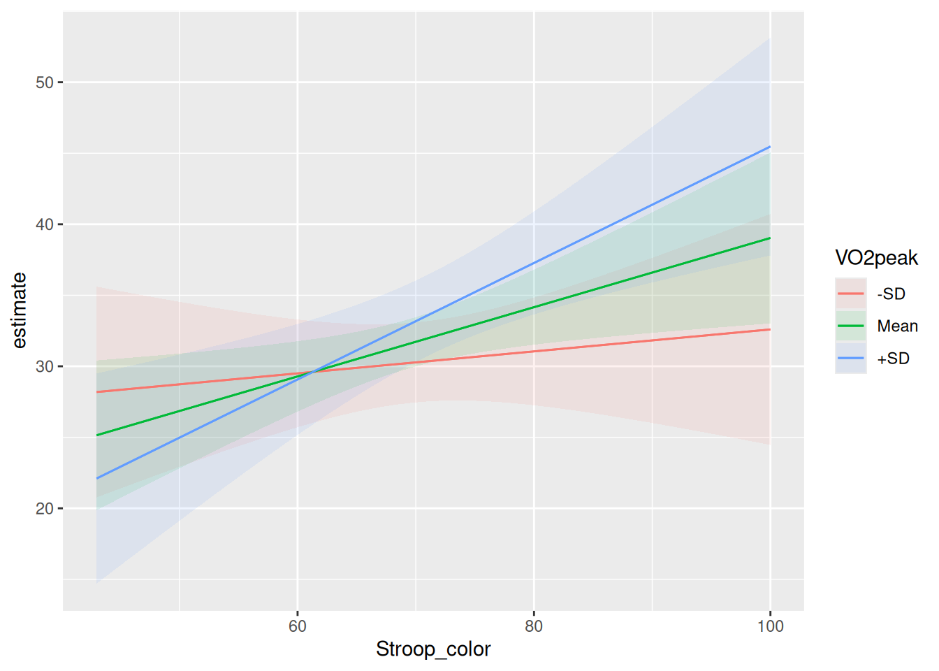
ImportantQuestion 4
- Interpret the plot for this interaction between Vo2Peak and Stroop Color.
After studying this example, it is you turn to find interactions:
ImportantQuestion 4
- Explore the possible combination of predictors and outcomes and try to find a possible interaction between two variables. You may follow the model found in Question 2.