Compare multiple models

Gaussian regression model

Author
Affiliation

Esteban Montenegro-Montenegro, PhD

Psychology and Child Development

Aims in this lecture

  • Introduce the concept of nested model.

  • Explain why we need to compare different statistical models?

  • Explain the concept of over-fitting a model.

  • And probably some memes…

Why do we care about model comparasion ?

  • As you might remember, probabilistic models are our possible explanations on how DATA is produced in Nature.

  • You may also recall that statistics is concerned with reducing uncertainty, specially because we always have unknown parameters in our models.

  • There could be multiple possible models that potentially explain how DATA is produced. We need to make a decision and select the model that best fit the DATA.

But wait… What is the best fit ?

  • You might be asking, what is a “fit” or “best fit” model?

  • When I’m using the word “fit”, I’m referring to how appropriate is the statistical model to explain the relationships of the outcome with all possible independent variables.

  • “Fit” also means that our model is an estimated model on observed data, therefore, our model could be a “good fit model” or “bad fit model”.

  • A bad fit model will not reproduce the most reliable estimates, and your standard errors will be large.

::: callout-important Remember: All models are wrong…but some are useful! (Box, 1976) :::

Let’s think about possible scenarios

  • Imagine that you have three independent variables that could be related to depression, let’s see the model:

\[depression \sim \beta_{0} + \beta_{1}selfEsteem_{1} + \beta_{2}likePancake_{2} + \beta_{3}rumination_{3} + \epsilon\]

  • In this model we have three predictors: 1) self-esteem score, 2) Do you like pancakes?, and a rumination score.

  • However, is this the best model? Would a model without \(\beta_{2}likePancake\) be a better fit model?

Model selection in the Classical Regression Model

\(R^2\) R-Square is not so boring

  • Commonly, we evaluate how good-fitted is hour regression model using the \(R^2\):

\[R^2 = \frac{SS_{M}}{SS_{t}}\] Where:

\(SS_{M}\) = Sum of Squares of the Model.

\(SS_{T}\) = Total Sum of Squares.

  • This should look similar to the estimation that we did when calculating an ANOVA model. Because, linear regression and ANOVA belong to the same family of the General Linear Model.

\(R^2\) R-Square is not so boring

  • You can see that \(R^2\) is a proportion of variance explained by the model. Why? Because, we divide the variability of the model by the total variability in the data. The result is an estimate that quantifies the percentage of variance explained by the model. As always, we can study an example:

\[depression \sim \beta_{0} + \beta_{1}selfEsteem_{1} + \beta_{2}numberCandies_{2} + \beta_{3}rumination_{3} + \epsilon\]

Show the code
### Simulation time!!
library(lavaan) ## <--- package to generate the values.
1
I’m specifying the “population model”.
2
This line creates the simulated values. I’m generating 100 random values.
3
Estimating the model using function lm().
This is lavaan 0.6-16.1856
lavaan is FREE software! Please report any bugs.
Show the code
library(broom)

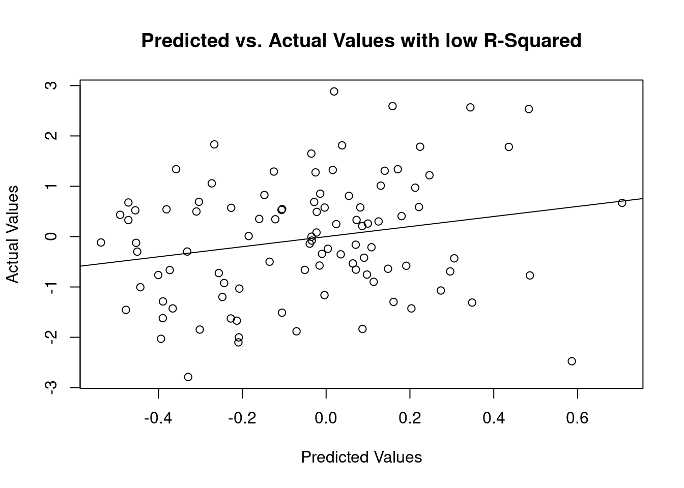
mod1 <- 'depression ~ 0.5*selfSteem + 0.8*rumination + 0*numberCandies'


generated <- simulateData(mod1,
                          meanstructure = TRUE, 
                          sample.nobs = 100,
                          seed = 12)


fitModel <- lm(depression ~ selfSteem + 
                 rumination + 
                 numberCandies, 
               data = generated)

gt(tidy(fitModel),
   rownames_to_stub= FALSE) |>
  fmt_number(decimals = 2)
term estimate std.error statistic p.value
(Intercept) −0.04 0.09 −0.41 0.68
selfSteem 0.37 0.10 3.80 0.00
rumination 0.75 0.10 7.81 0.00
numberCandies 0.03 0.09 0.28 0.78
  • Now let’s check the \(R^2\):
Show the code
gt(glance(fitModel) |>
     dplyr::select(r.squared, AIC, BIC)) |>
  fmt_number(decimals = 2) |>
  data_color(
    columns = c(r.squared),
    palette = "red")
r.squared AIC BIC
0.42 272.60 285.63
  • The \(R^2\) is 0.42, this can be read as: the linear model explains 42 % of the total variance.

\(R^2\) R-Square is not so boring

  • But, let’s see what happens when I delete the independent variable number of candies from the model:
Show the code
fitModel <- lm(depression ~ selfSteem + 
                 rumination, 
               data = generated)

gt(tidy(fitModel),
   rownames_to_stub= FALSE) |>
  fmt_number(decimals = 2)
1
In this example number of candies is omitted.
term estimate std.error statistic p.value
(Intercept) −0.04 0.09 −0.41 0.68
selfSteem 0.38 0.10 3.84 0.00
rumination 0.75 0.10 7.84 0.00
  • We can see again the \(R^2\):
Show the code
gt(glance(fitModel) |>
     dplyr::select(r.squared, AIC, BIC)) |>
  fmt_number(decimals = 2) |>
  data_color(
    columns = c(r.squared),
    palette = "red") |>
  tab_header(title = "R-squared after deleting number of candies")
R-squared after deleting number of candies
r.squared AIC BIC
0.42 270.68 281.10
  • So far, the \(R^2\) remained the same. It is an expected result, because number of candies was not explaining a portion of variance beyond chance.

  • But, if we delete a meaningful variable such as rumination the R^2 will decrease:

fitModel <- lm(depression ~ selfSteem + 
                 numberCandies, 
               data = generated)

gt(tidy(fitModel),
   rownames_to_stub= FALSE) |>
  fmt_number(decimals = 2) |>
  tab_header(title = "Estimated values after deleting rumination")
1
Rumination was deleted in this model.
Estimated values after deleting rumination
term estimate std.error statistic p.value
(Intercept) −0.06 0.12 −0.48 0.63
selfSteem 0.28 0.12 2.22 0.03
numberCandies 0.00 0.12 0.04 0.97
  • We can check again the \(R^2\) after deleting rumination:
Show the code
gt(glance(fitModel) |>
     dplyr::select(r.squared, AIC, BIC)) |>
  fmt_number(decimals = 2) |>
  data_color(
    columns = c(r.squared),
    palette = "red") |>
  tab_header(title = "R-squared after deleting rumination")
R-squared after deleting rumination
r.squared AIC BIC
0.05 319.76 330.18
  • You will see that the \(R^2\) value decreased after removing rumination. Why? Rumination is an important variable related to depression, by omitting rumination, your model explains less variance and therefore it affects the model fit.

Low vs. High \(R^2\)

fitModelHigh <- lm(depression ~ selfSteem + rumination +
                     numberCandies, 
                   data = generated)


plot(x=predict(fitModelHigh), y=generated$depression,
     xlab='Predicted Values',
     ylab='Actual Values',
     main='Predicted vs. Actual Values with high R-Squared')

abline(a=0, b=1)

Show the code
fitModelLow <- lm(depression ~ selfSteem + 
                    numberCandies, 
                  data = generated)


plot(x=predict(fitModelLow), y=generated$depression,
     xlab='Predicted Values',
     ylab='Actual Values',
     main='Predicted vs. Actual Values with low R-Squared')

abline(a=0, b=1)

Let’s get more serious…

It is a meme where terminator is all the options to select the best model, there is a cartoon that represents a psychology student hiding because she is scared of terminator.

More options to compare models

  • The \(R^2\) is an estimate that helps to select the best model. You will see that researchers select the model with a larger \(R^2\). But this is misleading.

  • The \(R^2\) could be inflated by adding non-meaningful predictors. If you throw multiple predictors into a regression you will get a high R-Squared. This is like doing a soup with random ingredients, you will probably get your soup but, is it the best soup?

More options to compare models

  • Akaike Information Criterion (AIC) is one of the alternatives to select variables, therefore we can arrive to the best fitted model possible.

  • The AIC was created by Hirotugu Akaike.

-Let’s see how this AIC fit measure looks like:

\[AIC = −2(\text{Log Likelihood}) + 2 \cdot ( \text{number of estimated parameters})\] - In the AIC estimation, you can see something call “Log Likelihood”. This is the information of the model. We haven’t had time to cover what is likelihood or something call “Maximum Likelihood”. But, at this point you are good if you understand “likelihood” as model information.

  • Number of estimated parameters is also part of the AIC estimation. This term in the estimation corresponds to how many parameter you are estimating in your model.
Tip

Parameter: unknown information in the model, we collect data to have information to reduce the uncertainty of the parameter or set of parameters.

  • We can understand the concept of number of parameters via an example:

\[depression \sim \beta_{0} + \beta_{1}selfEsteem_{1} + \beta_{2}numberCandies_{2} + \beta_{3}rumination_{3} + \epsilon\]

  • A few slides before, we studied the above model. If you count how many Greek letters it has, you will arrive to the total number of parameters:

  • We have three slopes represented by \(\beta_{i}\) (Beta).

  • We also have a residual error represented by \(\epsilon\).

  • We also have an intercept represented by \(\beta_{0}\).

  • Hence, we have in total 5 parameters!

More options to compare models

  • The AIC is considered a “penalized” information criterion. It will penalize models with a large number of parameters.

  • Lower values indicate a better fit model. While large values indicate poorly fitted models.

  • As always, take a look at the following example. I’m estimating a regression model where only the intercept of depression is estimated. In simple words, it is a model that is estimating only the mean of depression.

Show the code
ruminData <- read.csv("ruminationComplete.csv", 
                       na.strings = "99") |>
  mutate(ruminTotal = rowMeans(across(CRQS1:CRSQ13)),
         depreTotal = rowSums(across(CDI1:CDI26), na.rm = TRUE),
         anxTotal = rowMeans(across(DASS1:DASS7)),
         negativeBeliefs = rowMeans(across(NBRSdv1:NBRSdv13)),
         positiveBeliefs = rowMeans(across(PBRSdv1:PBRSdv9)),
         attention = ATENCION,
         activation = ACTIVACION)

#### We could estimate the most simple model.
#### This is a model that estimates only the intercept.

interceptOnly <- lm(depreTotal ~ 1, data = ruminData)

gt(tidy(interceptOnly),
   rownames_to_stub= FALSE) |>
  fmt_number(decimals = 2) |>
  tab_header(title = "Intercept-only model for the Depression score")
1
I’m reading in the data, then I’m computing the total score with mutate() function.
Intercept-only model for the Depression score
term estimate std.error statistic p.value
(Intercept) 10.44 0.43 24.12 0.00
  • The mean of depression according to the intercept-only model is 10.4433962. This model is so simple, because we didn’t add any predictor. This is what it makes this model a null model.

We can compare the null model

  • Now we are in good position to compare the intercept-only model versus alternative models. And guess what? We will use the AIC to compare alternative models.

  • We can start by adding one predictor, let’s add rumination:

Show the code
### Let's add rumination as a predictor.

fitWithRumination <- lm(depreTotal ~ ruminTotal, data = ruminData)

gt(tidy(fitWithRumination),
   rownames_to_stub= FALSE) |>
  fmt_number(decimals = 2) |>
  tab_header(title = "Rumination as predictor of the Depression score")
Rumination as predictor of the Depression score
term estimate std.error statistic p.value
(Intercept) −2.81 1.35 −2.08 0.04
ruminTotal 5.69 0.56 10.16 0.00
  • The result is not surprising, if you pay attention to the slope, we can say: For 1-point increment in rumination, depression increments 5.69 points. But, is this model a good fit for the data compare with the intercept-only model?
Show the code
compareAIC <- data.frame(Model = c("Intercept Model", 
                                   "Model adding Rumination"),
                         AICvalue = c(AIC(interceptOnly)[1], 
                                      AIC(fitWithRumination)[1]))

gt(compareAIC,
   rownames_to_stub= FALSE) |>
  fmt_number(decimals = 2) |>
  tab_header(title = "AIC values for the Intercept Model and the model with Rumination as predictor")
AIC values for the Intercept Model and the model with Rumination as predictor
Model AICvalue
Intercept Model 1,385.27
Model adding Rumination 1,259.84
  • The AIC value for the intercept model was higher compare to the model with one predictor. We can conclude that adding rumination helps to estimate a model that fits the data better.

Backward, and Forward variable selection: Building models

  • We just saw that AIC helps to select the best model, but what happens if you have multiple variables? Is there a way to select the best model faster? The answers is YES!

  • You can start adding one variable at the time, starting from the intercept-only model. In this approach you go “forward” by adding one variable at the time, then you compare each model versus the previous model.

  • You may also estimate a big model with multiple predictors. AIC can help you to trim the model until you keep the best variables related to your outcome. This is called “backwards” selection.

Backward, and Forward variable selection: Building models

  • In R you can use the function stepAIC() to select the best model with the best set of variables.

  • You can follow a forward selection process or a backwards selection process.

  • In the next example, I’ll start building all models using the forward method. The first model will be a model estimating only the intercept of depression, and at each step, the stepAIC() function will add one variable at the time, while comparing all the possible combination of models.

  • I’ll select the best model out of the following predictors:

    • Rumination.
    • Anxiety.
    • Negative metacognitive beliefs about rumination.
    • Positive metacognitive beliefs about rumination.
    • Activation.
    • Attention.
Show the code
library(MASS)

Attaching package: 'MASS'
The following object is masked from 'package:dplyr':

    select
Show the code
### Omit missing values

ruminDataNoMissing <- ruminData |>
  dplyr::select(depreTotal, 
         ruminTotal,
         anxTotal,
         negativeBeliefs,
         positiveBeliefs,
         attention,
         activation) |>
 drop_na()

interceptModel <- lm(depreTotal ~ 1, 
                     data = ruminDataNoMissing )

modelSelection <- stepAIC(interceptModel,
                          scope = list(upper = ~ruminTotal+anxTotal+negativeBeliefs+positiveBeliefs+attention+activation, 
                                       lower = ~1), 
                          direction = "forward",
                          trace = FALSE)


gt(tidy(modelSelection),
   rownames_to_stub= FALSE) |>
  fmt_number(decimals = 2) |>
  tab_header(title = "Final model selected by stepAIC")
Final model selected by stepAIC
term estimate std.error statistic p.value
(Intercept) −0.59 1.88 −0.31 0.76
ruminTotal 3.85 0.66 5.84 0.00
anxTotal 3.12 0.84 3.69 0.00
attention −0.25 0.08 −2.98 0.00
activation 0.21 0.09 2.25 0.03
negativeBeliefs 1.46 0.85 1.72 0.09
  • The final model selected by the stepAIC function was a model where positiveBeliefs is omitted. If we drop this variable we obtain the best set of variables to predict depression.
gt(modelSelection$anova,
   rownames_to_stub= FALSE) |>
  fmt_number(decimals = 2) |>
   cols_hide(columns = c(Df, Deviance, "Resid. Df", "Resid. Dev")) |>
  tab_header(title = "AIC values for all models forward method")
AIC values for all models forward method
Step AIC
715.80
+ ruminTotal 646.46
+ anxTotal 626.58
+ attention 624.43
+ activation 620.49
+ negativeBeliefs 619.46

In the table above, you can see all the AIC values estimated after adding one predictor at the time. The first step label is empty because there was not any predictor, it was an intercept-only model.

Backward, and Forward variable selection: Building models

  • A plot or multiple plots are always useful to interpret the results of the final best model:
library(marginaleffects)
library(patchwork)

Attaching package: 'patchwork'
The following object is masked from 'package:MASS':

    area
finalModel <- lm(depreTotal ~ ruminTotal+
                   anxTotal+
                   negativeBeliefs+
                   attention+
                   activation, 
                 data = ruminDataNoMissing)


rumPlot <- plot_predictions(finalModel, 
                       condition = c("ruminTotal"),
                 points = 0.5)

anxPlot <- plot_predictions(finalModel, 
                       condition = c("anxTotal"),
                 points = 0.5)

negativePlot <- plot_predictions(finalModel, 
                       condition = c("negativeBeliefs"),
                 points = 0.5)

attentionPlot <- plot_predictions(finalModel, 
                       condition = c("attention"),
                 points = 0.5)

activationPlot <- plot_predictions(finalModel, 
                       condition = c("activation"),
                 points = 0.5)

(rumPlot + anxPlot + negativePlot + attentionPlot)  + activationPlot

Backward, and Forward variable selection: Building models

  • The backwards procedure, will start with a full model and then, we can reduce the model based on the AIC measure. In the function stepAIC() you have to change direction = "forward" for direction = "backwards".

  • Following the previous example we can start with the full model:

Show the code
fullModel <- lm(depreTotal ~ ruminTotal+
                   anxTotal+
                   negativeBeliefs+
                   positiveBeliefs+
                   attention+
                   activation, 
                 data = ruminDataNoMissing)
1
The full model has all the predictors related to depression. The model will be reduced later.
  • Then, we can compare all the possible models using the function stepAIC():
Show the code
backwardsSelection <- stepAIC(interceptModel,
                          scope = list(upper = ~ruminTotal+anxTotal+negativeBeliefs+positiveBeliefs+attention+activation, 
                                       lower = ~1), 
                          direction = "backward",
                          trace = FALSE)
gt(tidy(backwardsSelection),
   rownames_to_stub= FALSE) |>
  fmt_number(decimals = 2) |>
  tab_header(title = "Final model selected by stepAIC backwards method0")
Final model selected by stepAIC backwards method0
term estimate std.error statistic p.value
(Intercept) 10.34 0.45 23.10 0.00

References

Box, G. E. (1976). Science and statistics. Journal of the American Statistical Association, 71(356), 791–799.