Brief introduction to Bayesian Structural Equation Modeling

Application in R using blavaan package

Esteban Montenegro-Montenegro, PhD

Department of Psychology and Child Development, CSU Stanislaus

2025-02-01

Aims in these two hours

Provide a short introduction to Structural Equation Modeling.
Introduce basic notions of Bayesian inference.
Jump into examples using the package blavaan in R.

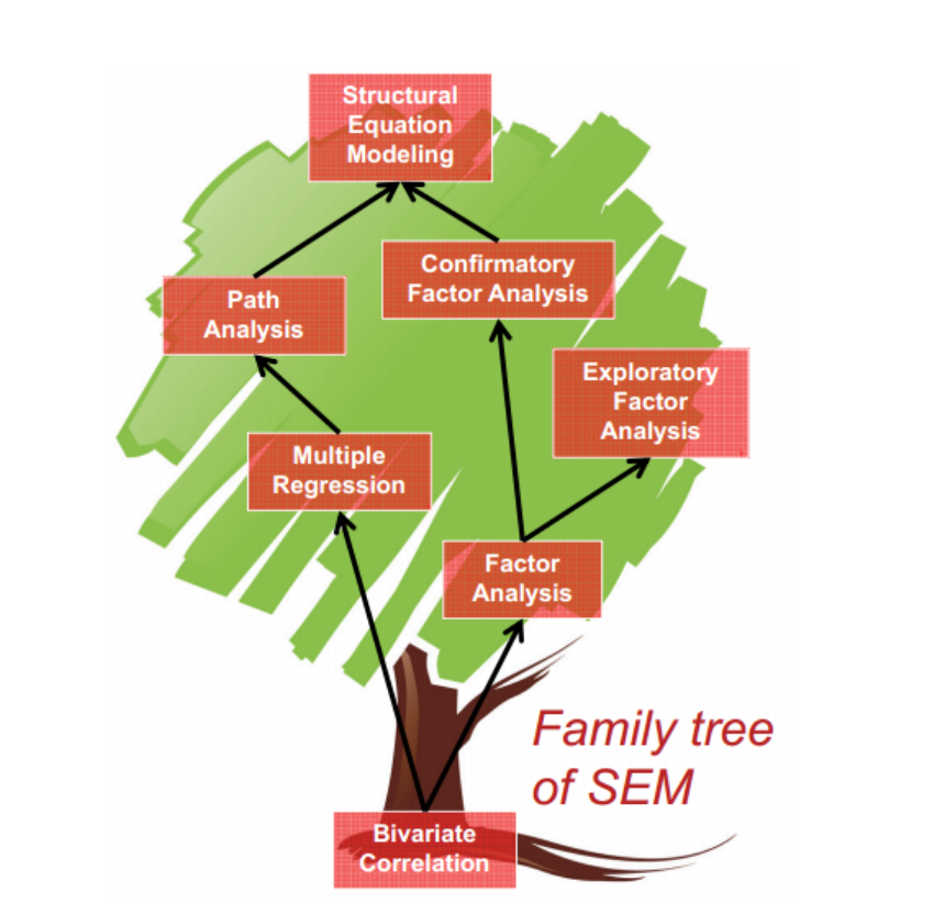
What is SEM ?

SEM is in reality a family of different possible models.
The roots of SEM are grounded in the notion of correlation and regression models.

SEM and latent variables

SEM is mostly used to estimate latent variables.
There are several definitions:

Bollen & Hoyle (2012):

Hypothetical variables.
Traits.
Data reduction strategy?
Classification strategy?
A variable in regression analysis which is, in principle
unmeasurable.

Have you thought how to measure intelligence?
What about the concept of “good performance”?
What does good health look like ? Is it a concept?

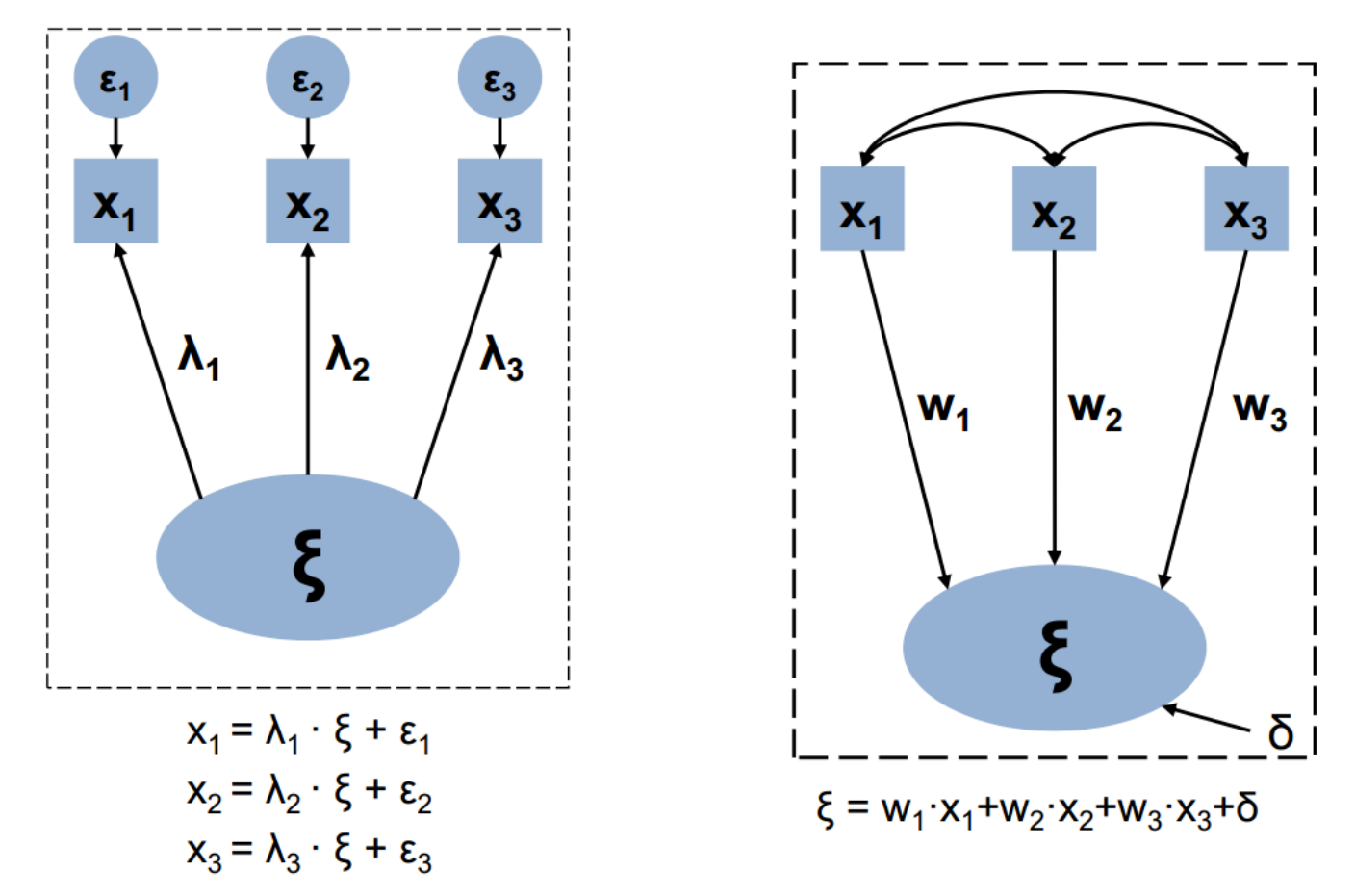
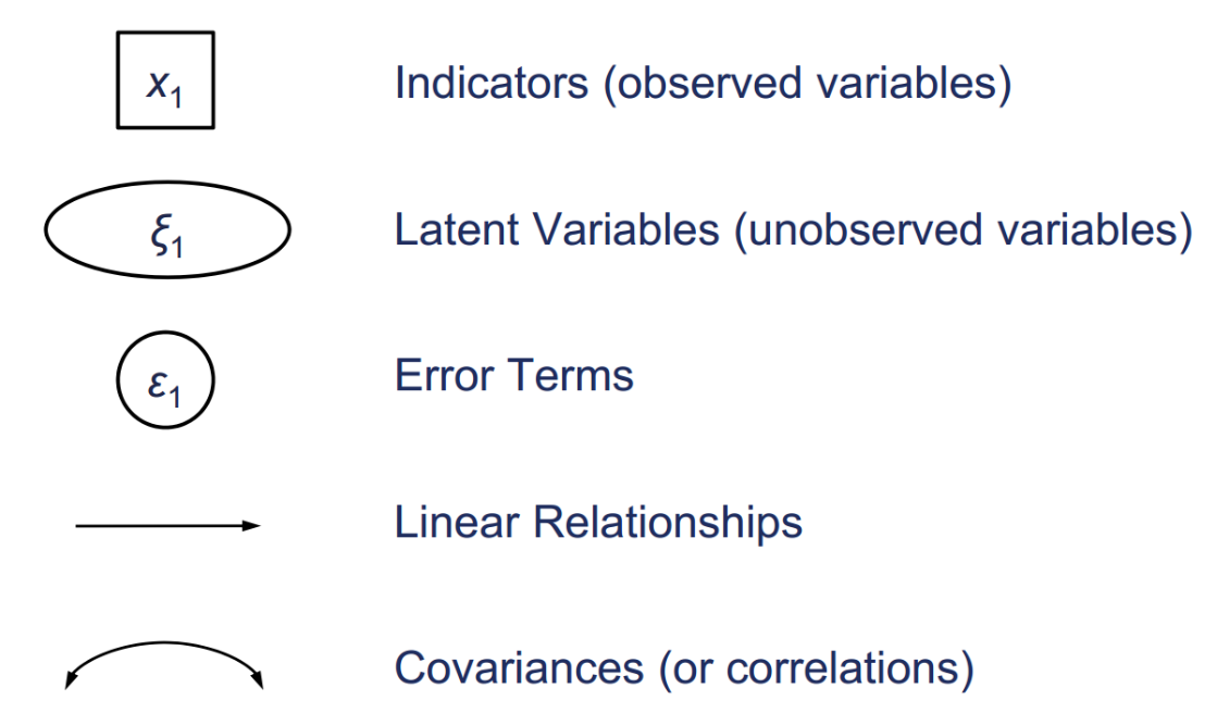
Let’s see the graphics convention

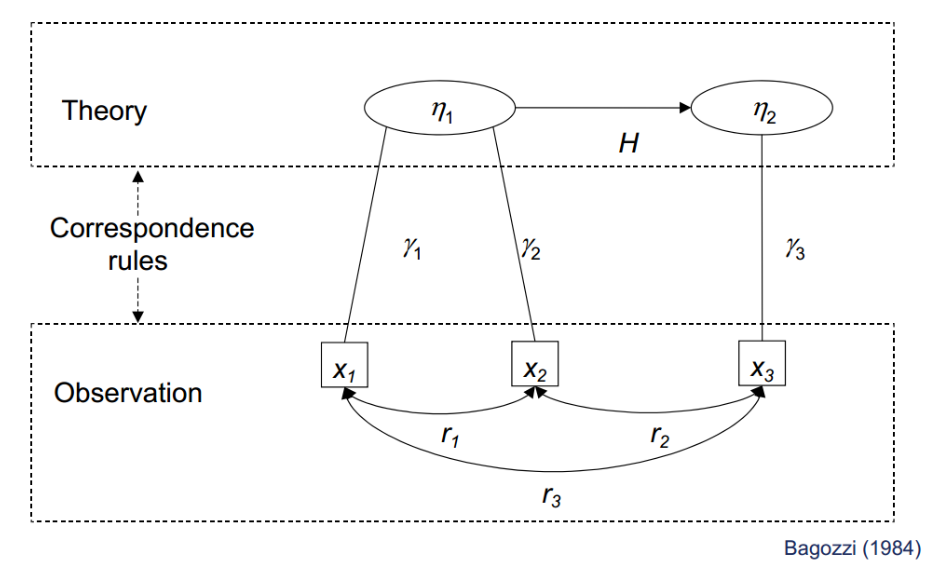
SEM relates to theories and ideas

Henseler (2020):

Reflective factors // Formative factors

Assumptions

Depends on how we estimate the model.
Multivariate normal data generating process.
Local independence: only the latent factor explains the indicators.
Sample size should be large enough to estimate the model.
Multicollinearity can be a problem.

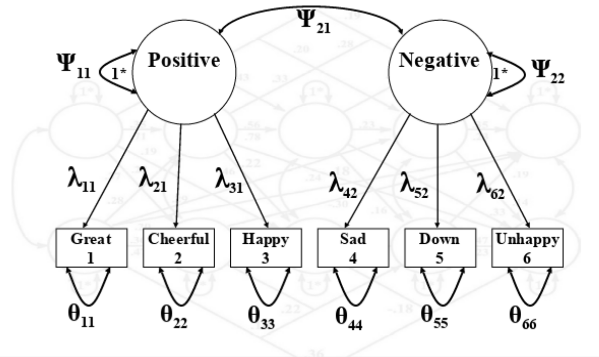
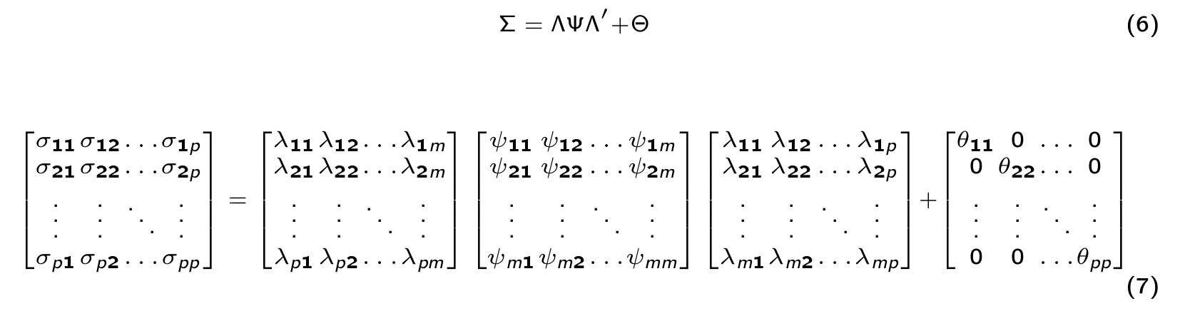
Let’s formally define the SEM model

\[\begin{equation} \Sigma = \Lambda \Psi \Lambda' + \Theta \end{equation}\]

Where:

\(\Sigma\) = The estimated covariance matrix.
\(\Psi\) = Matrix with covariance between latent factors.
\(\Lambda\) = Matrix with factor loadings.
\(\Theta\) = Matrix with unique observed variances.
In SEM we also have another model for the implied means:

\[\begin{equation} y = \tau + \Lambda\eta + \epsilon \end{equation}\]

Does it look familiar to you?

Let’s formally define the SEM model II

Model fit

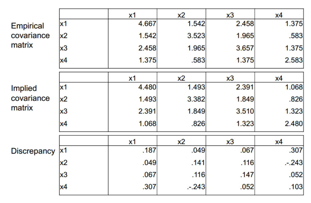
Most common fit measures

Root Mean Square Error of Approximation.

\[\begin{equation*} \label{eq:rmsea} \hat{\epsilon} = \sqrt{max \left[0, \frac{\chi^2_{ML} - df}{df(N)}\right]} = \sqrt{max \left[0, \frac{\chi^2_{ML} }{df} - \frac{1}{N}\right]} \end{equation*}\]

Tucker-Lewis Index (TLI)

\[\begin{equation*}\label{eq:tli} TLI = NNFI = \frac{\frac{\chi^2_{0}}{df_{0}}-\frac{\chi^2_{H}}{df_{H}}}{\frac{\chi^2_{0}}{df_{0}} -1} \end{equation*}\]

Comparative Fit Index (CFI)

\[\begin{equation} CFI = \frac{max(0, \hat{\lambda}_0) - max(0, \hat{\lambda}_H)}{max(0, \hat{\lambda}_0)} = 1 - \frac{max(0, \hat{\lambda}_H)}{max(0, \hat{\lambda}_0)} \end{equation}\]

Why should we use SEM ?

SEM has good properties:
- It helps to model several hypothesis at the same time.
- It has flexibility to estimate multigroup models.
- You have several estimators to choose.
- The model accounts for the error variance in your items.
- You can model non-linearity (we didn’t talk about it).
- You can estimate multilevel models.
- It is fun!

Let’s jump into Bayesian inference

Bayesian Rule

Bayesian inference helps to add uncertainty to your model.
Many researchers believe that Bayesian inference is only a strategy to add prior beliefs, but in reality the aim is to reflect in your model the level of uncertainty in your parameter estimation.

Bayesian Rule

\[\begin{equation*} p(\theta|y) = \frac{p(\theta,y)}{p(y)} = \frac{p(\theta)p(y|\theta)}{p(y)} \end{equation*}\]

Where:

prior distribution = \(p(\theta)\), and the sampling distribution = \(p(y|\theta)\) also called the likelihood of the data.

Bayesian Rule Example

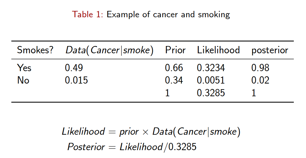
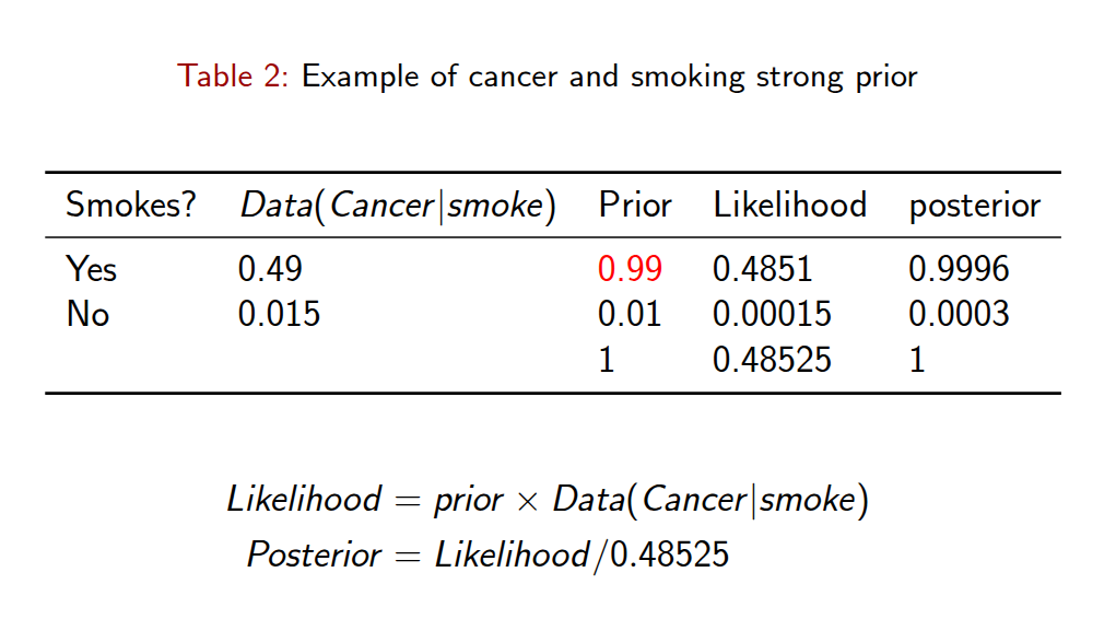
Frequentists vs. Bayesians

Frequentist: - “What is the likelihood of observing these data, given the parameter(s) of the model?”

Maximum likelihood methods basically work by iteratively finding values for q that maximize this function.

Bayesian:

“What is the distribution of the parameters, given the data?” A Bayesian is interested in how the parameters can be inferred from the data, not how the data would have been inferred from the parameters.

\[p(y|\theta)\]

In simple words …

Bayesian inference will help you to get a distribution for your parameters. This distribution is what we call the posterior distribution.
See the linear regression model:

\[\begin{equation*} Y = b_{0} + b_{1}X \end{equation*}\] \[\begin{align*} Y &\sim Normal(\mu, \sigma) \hspace{10.2em} [\text{likelihood}]\\ \mu &= b_{0} + b_{1}X \hspace{12.5em} [\text{equation}]\\ b_{0} & \sim normal(0,100) \hspace{10em} [\text{prior}]\\ b_{1} & \sim normal(0,100) \hspace{10em} [\text{prior}]\\ \sigma & \sim uniform(0,100) \hspace{9.4em} [\text{prior}]\\ \end{align*}\]

Let’s jump into Probability Density Function (pdf)

Bayesian is about probability distributions

Statistics in general is about probability distributions, however in Bayesian probability this is more explicit because each parameter will have a distribution.
This means, Bayesian assumes that there is a distribution for each parameter similar to the frequentist approach, but also Bayesian is able to generate a distribution for the parameters in your model. This is not feasible from the frequentist point of view.

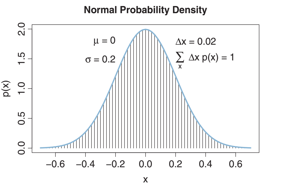
Multiple probability density functions in the universe

There is a multiverse of probability density functions

Model estimation in Bayesian inference

Estimation in Bayesian

This example is simple but in reality the estimation of Bayesian probability can be more complicated.
That’s why we need numerical algorithms.
Markov chain Monte Carlo (MCMC) is a group of algorithms
Given that we need to sample random values from the posterior distribution we need algorithms to make sure we don’t sample the same values too many times. We need to keep as many different values as possible.
There are different methods to estimate models in Bayesian inferences.
The most used method is Markov Chain Monte Carlo (MCMC) simulation.
In MCMC there are several samplers, the most used currently are:
- JAGS: Just Another Gibbs Sampler.
- Stan: No U-turn sampler (NUTS). Adaptive Hamiltonian Monte Carlo.
In the examples provided we are going to estimate models using the No U-turn sampler (NUTS) which is the default in Stan.
You may read more about samplers in Richard McElreath’s blog.

Why multiple chains?

When drawing possible values, we are also taking into account conditional relationships between parameters, and there are different states in the sampling process. Using multiple chains help to assess that no matter where the sampling starts in a conditional state, the generated values will remain very similar.

I’ll introduce an example using the package brms in R:

library(brms)

url <- "https://raw.githubusercontent.com/blackhill86/mm2/refs/heads/main/dataSets/ruminationClean.csv"

rumData <- read.csv(url)

modelRum<- brm(
  bf(depreZ ~ worryZ + rumZ),
  data = rumData ,
  family = gaussian(),
  chains = 3, 
  iter = 5000, 
  warmup = 2000,
  cores = 3, 
  seed = 1234,
)

See the results in plots

plot(modelRum)[1]

[[1]]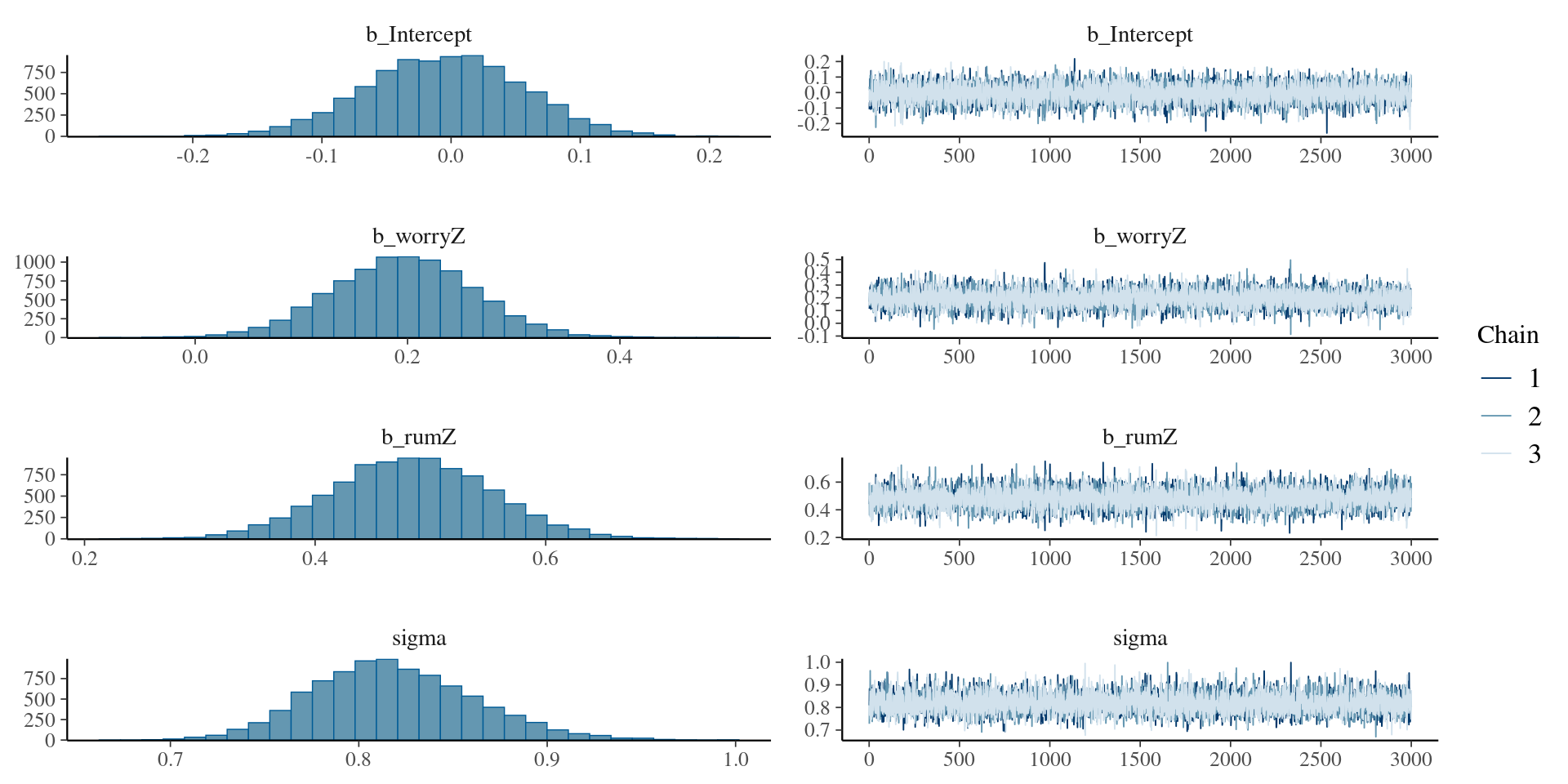

Let’s check further

summary(modelRum )

 Family: gaussian 
  Links: mu = identity; sigma = identity 
Formula: depreZ ~ worryZ + rumZ 
   Data: rumData (Number of observations: 186) 
  Draws: 3 chains, each with iter = 5000; warmup = 2000; thin = 1;
         total post-warmup draws = 9000

Regression Coefficients:
          Estimate Est.Error l-95% CI u-95% CI Rhat Bulk_ESS Tail_ESS
Intercept    -0.01      0.06    -0.12     0.11 1.00     8661     6344
worryZ        0.20      0.07     0.06     0.33 1.00     8010     7292
rumZ          0.48      0.07     0.35     0.62 1.00     8076     6674

Further Distributional Parameters:
      Estimate Est.Error l-95% CI u-95% CI Rhat Bulk_ESS Tail_ESS
sigma     0.82      0.04     0.74     0.91 1.00     8387     6664

Draws were sampled using sampling(NUTS). For each parameter, Bulk_ESS
and Tail_ESS are effective sample size measures, and Rhat is the potential
scale reduction factor on split chains (at convergence, Rhat = 1).

Let’s add a strong prior for fun

We can add a extremely dogmatic prior. We could believe that the distribution of our beta (\(\beta\)) parameters is \(\beta \sim N(0, 0.0001)\). Which means we believe the prior looks like this:

set.seed(123656)
plot(density(rnorm(n= 15000, mean = 0, sd = 0.0001)))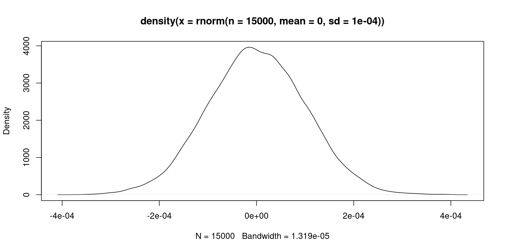

We can estimate this crazy idea:

modelRumStrong <- brm(
  bf(depreZ ~ worryZ + rumZ),
  data = rumData ,
  family = gaussian(),
  prior = set_prior("normal(0,0.001)", class = "b"),
  chains = 3, 
  iter = 5000, 
  warmup = 2000,
  cores = 3, 
  seed = 1234,
)

Let’s evaluate the result with plots

plot(modelRumStrong)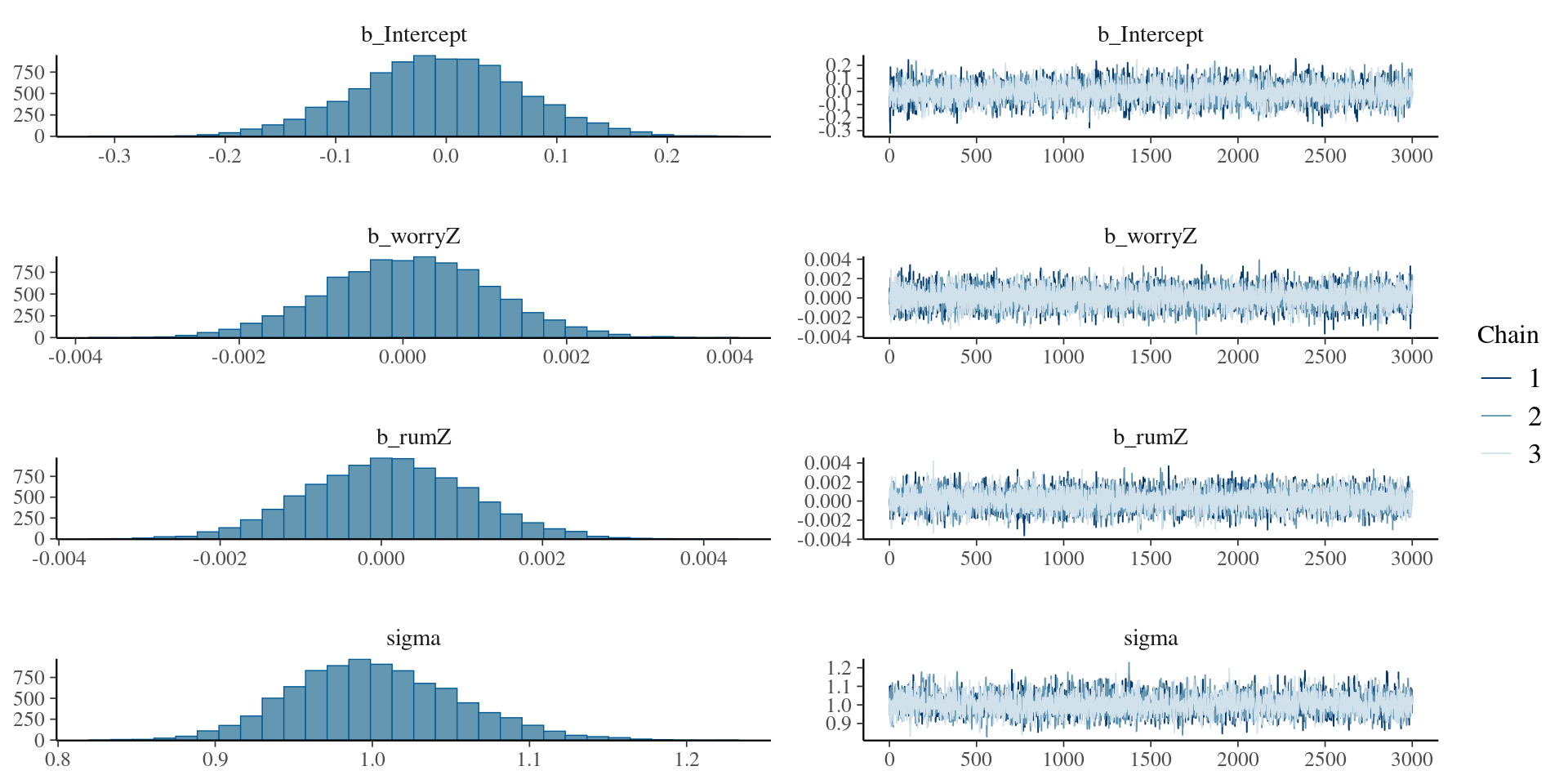

We can check it in a `summary` table

summary(modelRumStrong
        )

 Family: gaussian 
  Links: mu = identity; sigma = identity 
Formula: depreZ ~ worryZ + rumZ 
   Data: rumData (Number of observations: 186) 
  Draws: 3 chains, each with iter = 5000; warmup = 2000; thin = 1;
         total post-warmup draws = 9000

Regression Coefficients:
          Estimate Est.Error l-95% CI u-95% CI Rhat Bulk_ESS Tail_ESS
Intercept    -0.01      0.07    -0.16     0.14 1.00     5062     4505
worryZ        0.00      0.00    -0.00     0.00 1.00    11332     6676
rumZ          0.00      0.00    -0.00     0.00 1.00    10949     6630

Further Distributional Parameters:
      Estimate Est.Error l-95% CI u-95% CI Rhat Bulk_ESS Tail_ESS
sigma     1.00      0.05     0.90     1.11 1.00     4903     4801

Draws were sampled using sampling(NUTS). For each parameter, Bulk_ESS
and Tail_ESS are effective sample size measures, and Rhat is the potential
scale reduction factor on split chains (at convergence, Rhat = 1).

What happens in the case of SEM ?

SEM has many parameters compare to a regression model. You will see a distribution for each parameter, and depending on the complexity of the model it might take several minutes or hours to run. Also, if the model is not identified , you will see that the chains for some parameters will not converge.
However, BSEM is very useful when Maximum Likelihood has convergence problems and your model is identified. Complicated models will likely converge in SEM models.
Models with small sample sizes also will converge if the model is properly identified.
Also, it is easier in BSEM to regularize parameters, or try different approaches to test invariance such as approximate invariance.

Enought talking, let’s go to `R`…

References

Bollen, K. A., & Hoyle, R. H. (2012). Latent variables in structural equation modeling. In Handbook of structural equation modeling (pp. 56–67). The Guilford Press.

Henseler, J. (2020). Composite-based structural equation modeling: Analyzing latent and emergent variables. Guilford Publications.

Brief introduction to Bayesian Structural Equation Modeling

Aims in these two hours

What is SEM ?

SEM and latent variables

Let’s see the graphics convention

Let’s see the graphics convention

SEM relates to theories and ideas

Reflective factors // Formative factors

Assumptions

Let’s formally define the SEM model

Let’s formally define the SEM model II

Model fit

Most common fit measures

Why should we use SEM ?

Let’s jump into Bayesian inference

Bayesian Rule

Bayesian Rule

Bayesian Rule Example

Frequentists vs. Bayesians

In simple words …

Let’s jump into Probability Density Function (pdf)

Bayesian is about probability distributions

Multiple probability density functions in the universe

Model estimation in Bayesian inference

Estimation in Bayesian

Why multiple chains?

See the results in plots

Let’s check further

Let’s add a strong prior for fun

Let’s evaluate the result with plots

We can check it in a summary table

What happens in the case of SEM ?

Enought talking, let’s go to R…

References

We can check it in a `summary` table

Enought talking, let’s go to `R`…